Chapter 12 Utbildningsnivå
Befolkning efter region, ålder, utbildningsnivå, kön och år ålder 16-74 år kön män och kvinnor år 2017
utb <- readfile("UF0506A1.csv")
utb$utbildningsnivå <- as.factor(utb$utbildningsnivå)
utb$utbildningsnivå <- factor(utb$utbildningsnivå, levels(utb$utbildningsnivå)[c(3, 1, 2, 6, 7, 5, 4, 8)])
utb %>%
  filter (utbildningsnivå != "uppgift om utbildningsnivå saknas") %>%
  mutate(lnkod_n = substr(region, 1,2)) %>%
  ggplot(aes(x = lnkod_n, y = salary, fill = utbildningsnivå)) +
    geom_col(position = "fill") +
    theme(legend.position="bottom") +
facet_grid(. ~ kön) 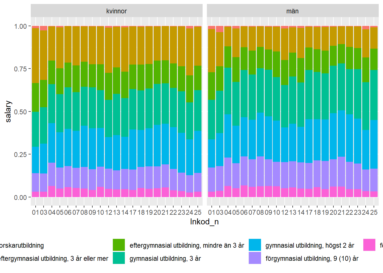
Figure 12.1: Education distribution in different counties.
readfile("UF0506A1.csv") %>%
  group_by(utbildningsnivå, region, kön) %>%
  mutate(utbregno = sum(salary)) %>%
  group_by(region) %>% mutate(perc = utbregno / sum(utbregno)) %>%
  filter (utbildningsnivå == "eftergymnasial utbildning, 3 år eller mer") %>%
  mutate(lnkod_n = as.numeric(substr(region, 1,2))) %>%
  right_join(map_ln_n, by = "lnkod_n") %>%
  ggplot() +
    geom_polygon(mapping = aes(x = ggplot_long, y = ggplot_lat, group = lnkod, fill = perc)) +
    coord_equal() +
facet_grid(. ~ kön) 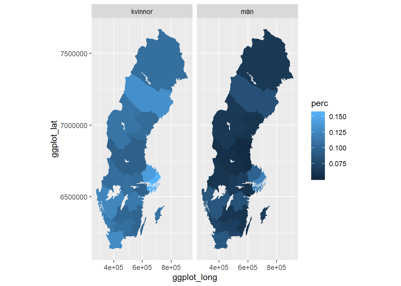
Figure 12.2: Percentage of the population who have 3 years or more post-secondary education, but not postgraduate education.
readfile("UF0506A1.csv") %>%
  group_by(utbildningsnivå, region) %>%
  summarize(utbregno = sum(salary)) %>%
  group_by(region) %>% mutate(perc = utbregno / sum(utbregno)) %>%
  filter (utbildningsnivå == "eftergymnasial utbildning, 3 år eller mer") %>%
  mutate(lnkod_n = as.numeric(substr(region, 1,2))) %>%
  right_join(salary_2017, by = c("lnkod_n" = "Länskod")) %>%
  ggscatter(x = "salary", y = "perc",
    add = "reg.line", conf.int = TRUE,
    cor.coef = TRUE, cor.method = "pearson") +
    labs(
      x = "Salary (SEK)",
      y = "Percent with 3 years post-secondary education"
    )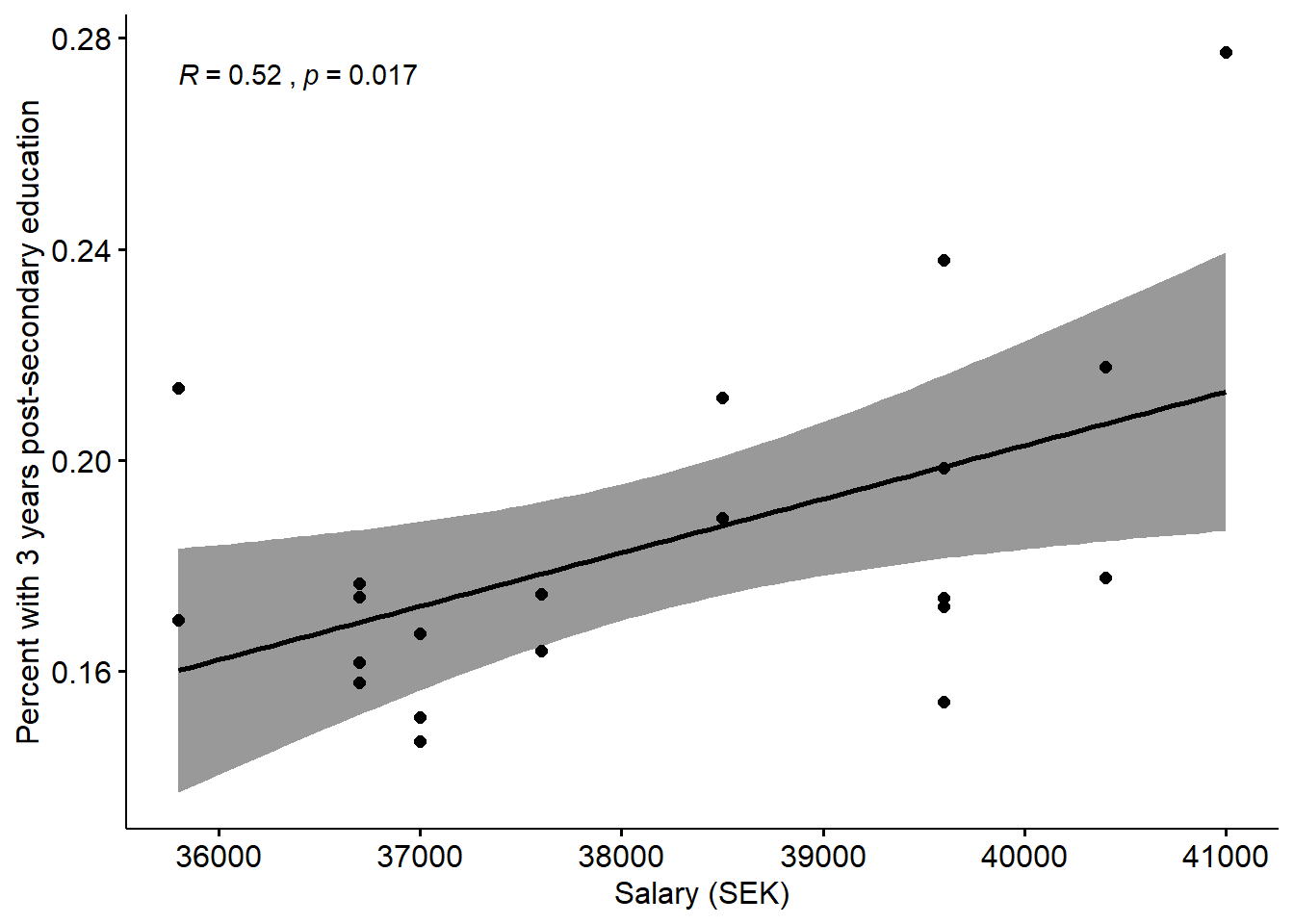
Figure 12.3: The correlation between the proportion of the population who have 3 years or more post-secondary education, but not postgraduate education, and the salaries of engineers in the region.
12.1 The correlation between the proportion of engineers who are women and the number of the population who have 3 years or more post-secondary education in the region. Year 2014 - 2018
Average basic salary, monthly salary and women´s salary as a percentage of men´s salary by region, sector, occupational group (SSYK 2012) and sex . Year 2014 - 2018 Monthly salaty All sectors 214 Engineering professionals
Average basic salary, monthly salary and women´s salary as a percentage of men´s salary by region, sector, occupational group (SSYK 2012) and sex . Year 2014 - 2018 Number of employees All sectors 214 Engineering professionals
Population 16-74 years of age by region, highest level of education, age and sex. The year 1985 - 2018. total 16-74 years
tb <- readfile("000000CG_10.csv")
tb <- readfile("000000CD_10.csv") %>%
  left_join(tb, by = c("region", "year", "sex")) %>%
  group_by (`region`, year) %>%
  mutate (perc_women = as.numeric (sub ("%", "", perc_women (salary.x)))) %>%
  mutate (perc_salary = as.numeric (sub ("%", "", perc_sal (salary.y)))) %>%
  mutate (sum_ing = sum(salary.x))
readfile("UF0506A1_1.csv") %>%
  group_by(`level of education`, region, year, sex) %>%
  mutate(utbregno = sum(salary)) %>%
  group_by(region, year, sex) %>% mutate(perc_edu = utbregno / sum(utbregno)) %>%
  group_by(`level of education`, region, year) %>%
  mutate (sum_edu = sum(utbregno)) %>%
  filter (`level of education` == "post-secondary education 3 years or more (ISCED97 5A)") %>%
  right_join(tb, by = c("region", "year", "sex")) %>%
  mutate (perc_eng = sum_ing / sum_edu) %>%
  ggplot(aes(x = sum_edu, y = perc_women, colour = region, size = year2)) +
  geom_point() +
  theme(legend.position="bottom") +
  labs(
    x = "Number of the population with 3 years or more post-secondary education",
    y = "Per cent of engineers who are women"
  )
## Warning: Removed 2 rows containing missing values (geom_point).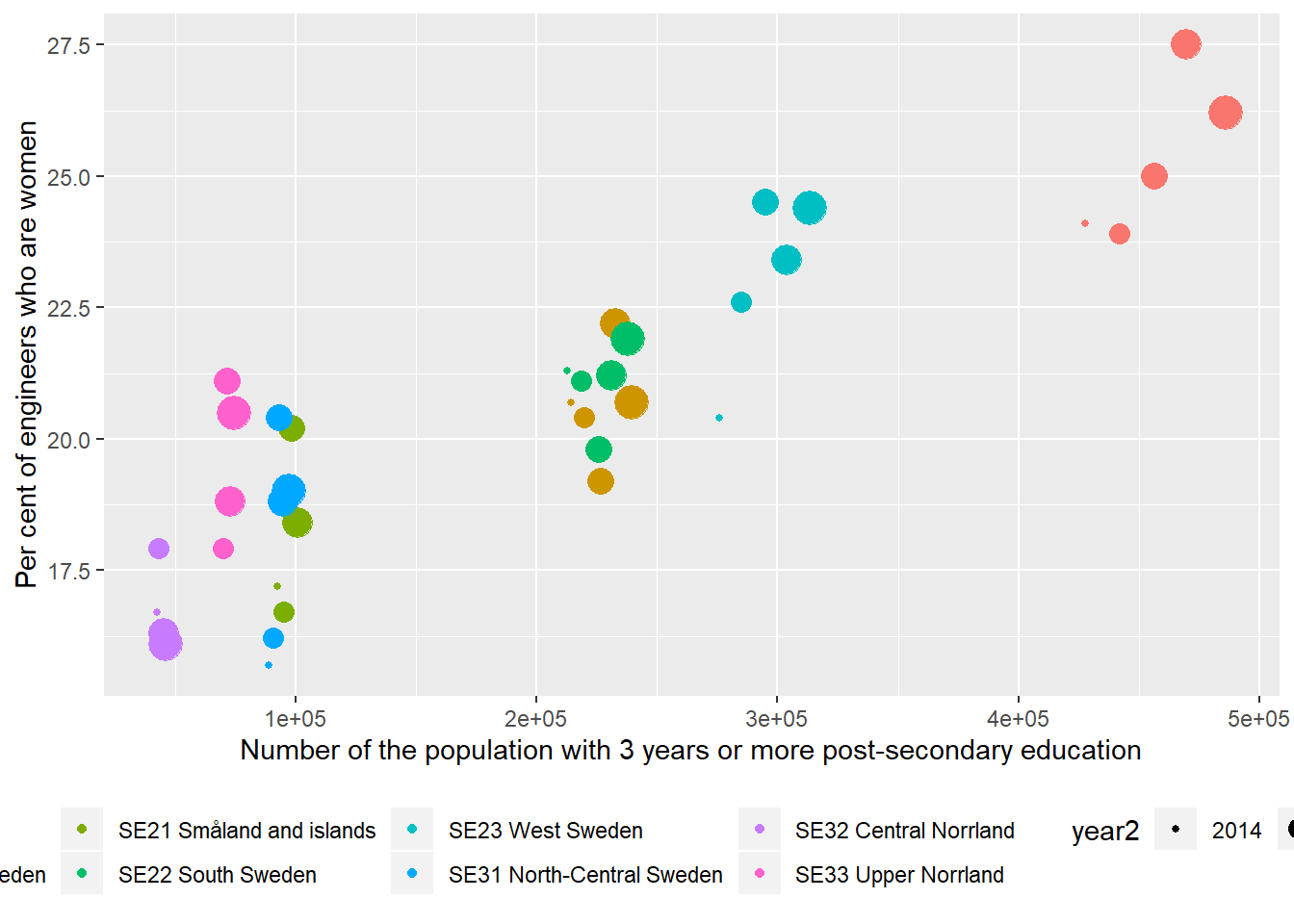
Figure 12.4: The correlation between the proportion of engineers who are women and the number of the population who have 3 years or more post-secondary education, but not postgraduate education in the regions (NUTS2), Year 2014 - 2018.
tb <- readfile("000000CG_10.csv")
tb <- readfile("000000CD_10.csv") %>%
  left_join(tb, by = c("region", "year", "sex")) %>%
  group_by (`region`, year) %>%
  mutate (perc_women = as.numeric (sub ("%", "", perc_women (salary.x)))) %>%
  mutate (perc_salary = as.numeric (sub ("%", "", perc_sal (salary.y)))) %>%
  mutate (sum_ing = sum(salary.x))
readfile("UF0506A1_1.csv") %>%
  group_by(`level of education`, region, year, sex) %>%
  mutate(utbregno = sum(salary)) %>%
  group_by(region, year, sex) %>% mutate(perc_edu = utbregno / sum(utbregno)) %>%
  group_by(`level of education`, region, year) %>%
  mutate (sum_edu = sum(utbregno)) %>%
  filter (`level of education` == "post-secondary education 3 years or more (ISCED97 5A)") %>%
  right_join(tb, by = c("region", "year", "sex")) %>%
  mutate (perc_eng = sum_ing / sum_edu) %>%
  ggscatter(x = "sum_edu", y = "perc_women",
  add = "reg.line", conf.int = TRUE,
  cor.coef = TRUE, cor.method = "pearson") +
  labs(
    x = "Number of the population with 3 years or more post-secondary education",
    y = "Per cent of engineers who are women"
  )
## Warning: Removed 2 rows containing non-finite values (stat_smooth).## Warning: Removed 2 rows containing non-finite values (stat_cor).## Warning: Removed 2 rows containing missing values (geom_point).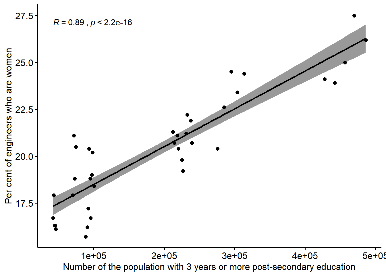
Figure 12.5: The correlation between the proportion of engineers who are women and the number of the population who have 3 years or more post-secondary education, but not postgraduate education in the regions (NUTS2), Year 2014 - 2018.
tb <- readfile("000000CG_10.csv")
tb <- readfile("000000CD_10.csv") %>%
  left_join(tb, by = c("region", "year", "sex")) %>%
  group_by (`region`, year) %>%
  mutate (perc_women = as.numeric (sub ("%", "", perc_women (salary.x)))) %>%
  mutate (perc_salary = as.numeric (sub ("%", "", perc_sal (salary.y)))) %>%
  mutate (sum_ing = sum(salary.x))
tb <- readfile("UF0506A1_1.csv") %>%
  group_by(`level of education`, region, year, sex) %>%
  mutate(utbregno = sum(salary)) %>%
  group_by(region, year, sex) %>% mutate(perc_edu = utbregno / sum(utbregno)) %>%
  group_by(region, year) %>% mutate(sum_pop = sum(utbregno)) %>%
  group_by(`level of education`, region, year) %>%
  mutate (sum_edu = sum(utbregno)) %>%
  right_join(tb, by = c("region", "year", "sex")) %>%
  mutate (perc_eng = sum_ing / sum_edu) %>%
  filter (`level of education` == "post-secondary education 3 years or more (ISCED97 5A)")

model <- lm(perc_women ~ sum_edu + year2 + log(salary.y), data = tb)

summary(model) %>%
  tidy() %>%
  knitr::kable(
  booktabs = TRUE,
caption = 'Women engineers and population with 3 years or more post-secondary education')| term | estimate | std.error | statistic | p.value |
|---|---|---|---|---|
| (Intercept) | -885.3287385 | 229.7997838 | -3.852609 | 0.0002512 |
| sum_edu | 0.0000214 | 0.0000016 | 13.652812 | 0.0000000 |
| year2 | 0.4719358 | 0.1228379 | 3.841941 | 0.0002604 |
| log(salary.y) | -4.6839227 | 3.6243664 | -1.292342 | 0.2003709 |
Anova(model, type=2) %>%
  tidy() %>%
  knitr::kable(
  booktabs = TRUE,
caption = 'Anova report from linear model fit') | term | sumsq | df | statistic | p.value |
|---|---|---|---|---|
| sum_edu | 292.335537 | 1 | 186.399278 | 0.0000000 |
| year2 | 23.149348 | 1 | 14.760510 | 0.0002604 |
| log(salary.y) | 2.619345 | 1 | 1.670149 | 0.2003709 |
| Residuals | 112.919744 | 72 | NA | NA |
12.2 The correlation between the number of engineers and the number of the population who have 3 years or more post-secondary education in the regions, Year 2014 - 2018.
tb <- readfile("000000CG_10.csv")
tb <- readfile("000000CD_10.csv") %>%
  left_join(tb, by = c("region", "year", "sex")) %>%
  group_by (`region`, year) %>%
  mutate (perc_women = as.numeric (sub ("%", "", perc_women (salary.x)))) %>%
  mutate (perc_salary = as.numeric (sub ("%", "", perc_sal (salary.y)))) %>%
  mutate (sum_ing = sum(salary.x))
readfile("UF0506A1_1.csv") %>%
  group_by(`level of education`, region, year, sex) %>%
  mutate(utbregno = sum(salary)) %>%
  group_by(region, year, sex) %>% mutate(perc_edu = utbregno / sum(utbregno)) %>%
  group_by(`level of education`, region, year) %>%
  mutate (sum_edu = sum(utbregno)) %>%
  filter (`level of education` == "post-secondary education 3 years or more (ISCED97 5A)") %>%
  right_join(tb, by = c("region", "year", "sex")) %>%
  mutate (perc_eng = sum_ing / sum_edu) %>%
  ggplot(aes(x = sum_edu, y = sum_ing, colour = region, size = year2)) +
  geom_point() +
  theme(legend.position="bottom") +
  labs(
    x = "Number of the population with 3 years or more post-secondary education",
    y = "Number of the population who are engineers"
  )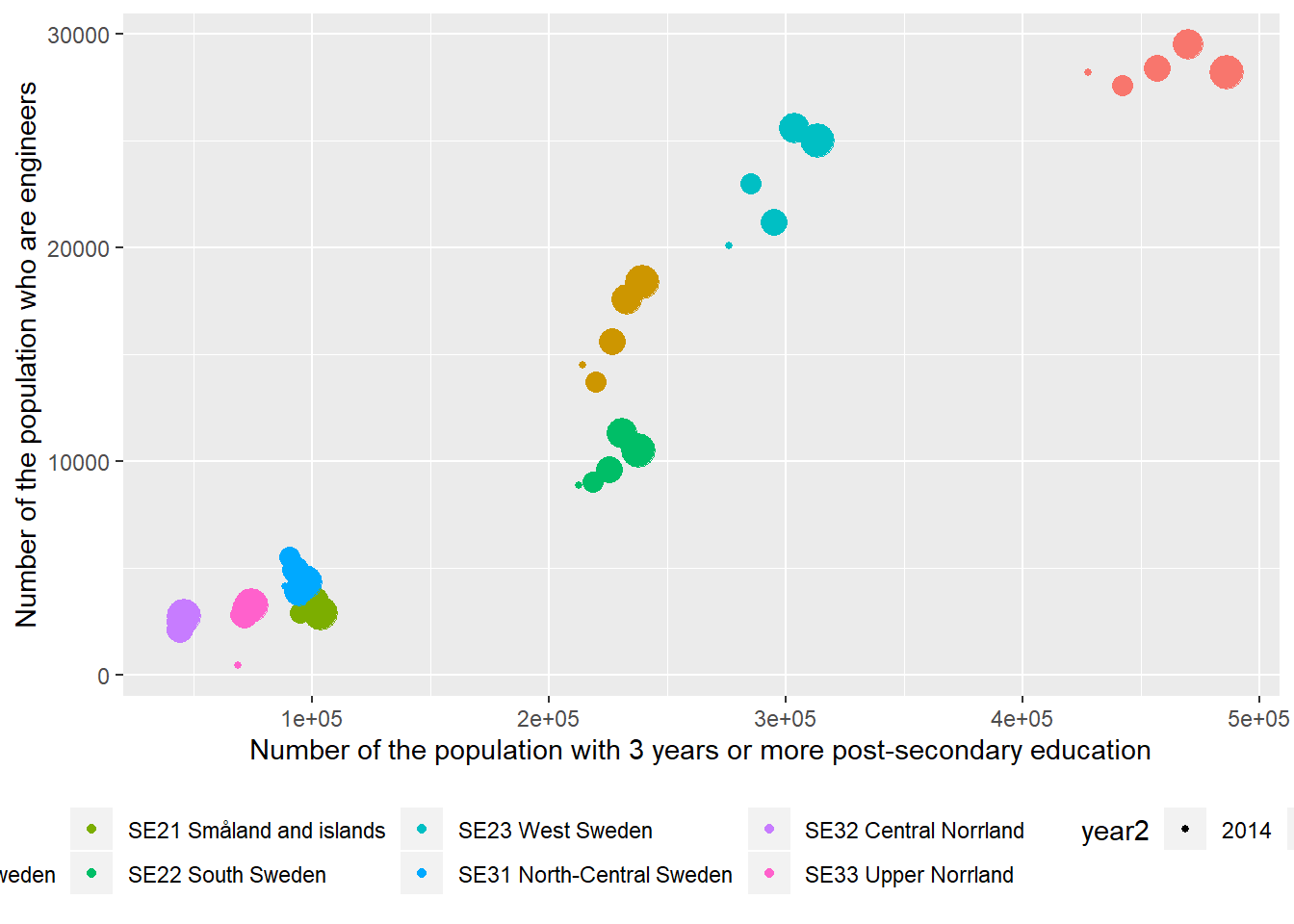
Figure 12.6: The correlation between the number of engineers and the number of the population who have 3 years or more post-secondary education, but not postgraduate education in the regions (NUTS2), Year 2014 - 2018.
tb <- readfile("000000CG_10.csv")
tb <- readfile("000000CD_10.csv") %>%
  left_join(tb, by = c("region", "year", "sex")) %>%
  group_by (`region`, year) %>%
  mutate (perc_women = as.numeric (sub ("%", "", perc_women (salary.x)))) %>%
  mutate (perc_salary = as.numeric (sub ("%", "", perc_sal (salary.y)))) %>%
  mutate (sum_ing = sum(salary.x))
readfile("UF0506A1_1.csv") %>%
  group_by(`level of education`, region, year, sex) %>%
  mutate(utbregno = sum(salary)) %>%
  group_by(region, year, sex) %>% mutate(perc_edu = utbregno / sum(utbregno)) %>%
  group_by(`level of education`, region, year) %>%
  mutate (sum_edu = sum(utbregno)) %>%
  filter (`level of education` == "post-secondary education 3 years or more (ISCED97 5A)") %>%
  right_join(tb, by = c("region", "year", "sex")) %>%
  mutate (perc_eng = sum_ing / sum_edu) %>%
  ggscatter(x = "sum_edu", y = "sum_ing",
  add = "reg.line", conf.int = TRUE,
  cor.coef = TRUE, cor.method = "pearson") +
  labs(
    x = "Number of the population with 3 years or more post-secondary education",
    y = "Number of the population who are engineers"
  )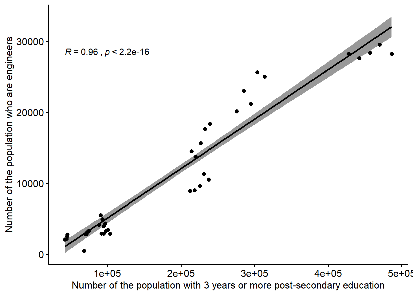
Figure 12.7: The correlation between the number of engineers and the number of the population who have 3 years or more post-secondary education, but not postgraduate education in the regions (NUTS2), Year 2014 - 2018.
tb <- readfile("000000CG_10.csv")
tb <- readfile("000000CD_10.csv") %>%
  left_join(tb, by = c("region", "year", "sex")) %>%
  group_by (`region`, year) %>%
  mutate (perc_women = as.numeric (sub ("%", "", perc_women (salary.x)))) %>%
  mutate (perc_salary = as.numeric (sub ("%", "", perc_sal (salary.y)))) %>%
  mutate (sum_ing = sum(salary.x))
tb <- readfile("UF0506A1_1.csv") %>%
  group_by(`level of education`, region, year, sex) %>%
  mutate(utbregno = sum(salary)) %>%
  group_by(region, year, sex) %>% mutate(perc_edu = utbregno / sum(utbregno)) %>%
  group_by(region, year) %>% mutate(sum_pop = sum(utbregno)) %>%
  group_by(`level of education`, region, year) %>%
  mutate (sum_edu = sum(utbregno)) %>%
  right_join(tb, by = c("region", "year", "sex")) %>%
  mutate (perc_eng = sum_ing / sum_edu) %>%
  filter (`level of education` == "post-secondary education 3 years or more (ISCED97 5A)")

model <- lm(sum_edu ~ year2 + log(salary.y) * sum_pop, data = tb)

summary(model) %>%
  tidy() %>%
  knitr::kable(
  booktabs = TRUE,
caption = 'Population with 3 years or more post-secondary education and number of population')| term | estimate | std.error | statistic | p.value |
|---|---|---|---|---|
| (Intercept) | 5.129274e+06 | 5.118336e+06 | 1.0021372 | 0.3195877 |
| year2 | 1.213056e+02 | 2.669735e+03 | 0.0454373 | 0.9638828 |
| log(salary.y) | -5.089895e+05 | 1.206615e+05 | -4.2183249 | 0.0000698 |
| sum_pop | -7.867544e+00 | 1.172156e+00 | -6.7120268 | 0.0000000 |
| log(salary.y):sum_pop | 7.616666e-01 | 1.099515e-01 | 6.9272996 | 0.0000000 |
Anova(model, type=2) %>%
  tidy() %>%
  knitr::kable(
  booktabs = TRUE,
caption = 'Anova report from linear model fit') | term | sumsq | df | statistic | p.value |
|---|---|---|---|---|
| year2 | 1490425 | 1 | 0.0020646 | 0.9638828 |
| log(salary.y) | 2556263146 | 1 | 3.5409595 | 0.0638575 |
| sum_pop | 567943896187 | 1 | 786.7211812 | 0.0000000 |
| log(salary.y):sum_pop | 34642763902 | 1 | 47.9874796 | 0.0000000 |
| Residuals | 52699616348 | 73 | NA | NA |
12.3 The correlation between the number of engineers and the proportion of engineers who are women in the regions, Year 2014 - 2018
tb <- readfile("000000CG_10.csv")
tb <- readfile("000000CD_10.csv") %>%
  left_join(tb, by = c("region", "year", "sex")) %>%
  group_by (`region`, year) %>%
  mutate (perc_women = as.numeric (sub ("%", "", perc_women (salary.x)))) %>%
  mutate (perc_salary = as.numeric (sub ("%", "", perc_sal (salary.y)))) %>%
  mutate (sum_ing = sum(salary.x))
readfile("UF0506A1_1.csv") %>%
  group_by(`level of education`, region, year, sex) %>%
  group_by(`level of education`, region, year, sex) %>%
  mutate(utbregno = sum(salary)) %>%
  group_by(region, year, sex) %>% mutate(perc_edu = utbregno / sum(utbregno)) %>%
  group_by(`level of education`, region, year) %>%
  mutate (sum_edu = sum(utbregno)) %>%
  filter (`level of education` == "post-secondary education 3 years or more (ISCED97 5A)") %>%
  right_join(tb, by = c("region", "year", "sex")) %>%
  mutate (perc_eng = sum_ing / sum_edu) %>%
  ggplot(aes(x = perc_women, y = sum_ing, colour = region, size = year2)) +
  geom_point() +
  theme(legend.position="bottom") +
  labs(
    x = "Per cent of engineers who are women",
    y = "Number of the population who are engineers"
  )
## Warning: Removed 2 rows containing missing values (geom_point).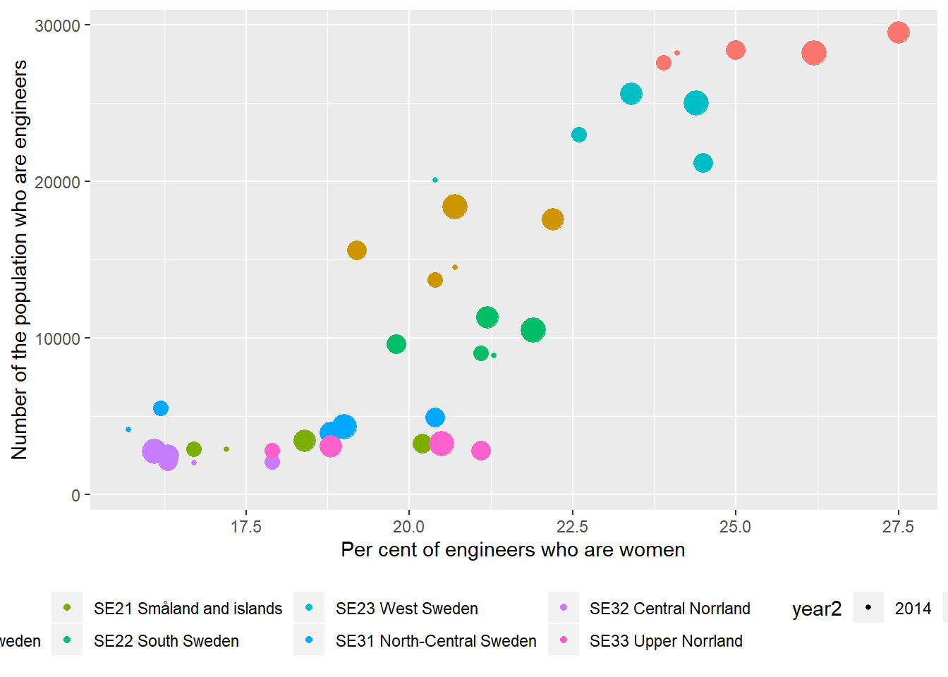
Figure 12.8: The correlation between the number of engineers and the proportion of engineers who are women in the regions (NUTS2), Year 2014 - 2018.
tb <- readfile("000000CG_10.csv")
tb <- readfile("000000CD_10.csv") %>%
  left_join(tb, by = c("region", "year", "sex")) %>%
  group_by (`region`, year) %>%
  mutate (perc_women = as.numeric (sub ("%", "", perc_women (salary.x)))) %>%
  mutate (perc_salary = as.numeric (sub ("%", "", perc_sal (salary.y)))) %>%
  mutate (sum_ing = sum(salary.x))
readfile("UF0506A1_1.csv") %>%
  group_by(`level of education`, region, year, sex) %>%
  group_by(`level of education`, region, year, sex) %>%
  mutate(utbregno = sum(salary)) %>%
  group_by(region, year, sex) %>% mutate(perc_edu = utbregno / sum(utbregno)) %>%
  group_by(`level of education`, region, year) %>%
  mutate (sum_edu = sum(utbregno)) %>%
  filter (`level of education` == "post-secondary education 3 years or more (ISCED97 5A)") %>%
  right_join(tb, by = c("region", "year", "sex")) %>%
  mutate (perc_eng = sum_ing / sum_edu) %>%
  ggscatter(x = "perc_women", y = "sum_ing",
  add = "reg.line", conf.int = TRUE,
  cor.coef = TRUE, cor.method = "pearson") +
  labs(
    x = "Per cent of engineers who are women",
    y = "Number of the population who are engineers"
  )
## Warning: Removed 2 rows containing non-finite values (stat_smooth).## Warning: Removed 2 rows containing non-finite values (stat_cor).## Warning: Removed 2 rows containing missing values (geom_point).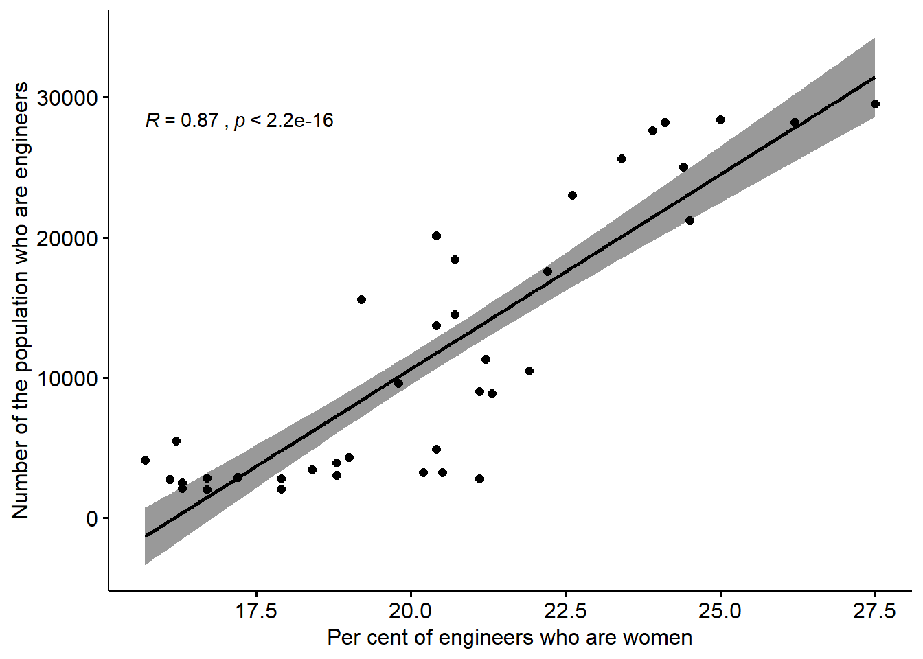
Figure 12.9: The correlation between the number of engineers and the proportion of engineers who are women in the regions (NUTS2), Year 2014 - 2018.
tb <- readfile("000000CG_10.csv")
tb <- readfile("000000CD_10.csv") %>%
  left_join(tb, by = c("region", "year", "sex")) %>%
  group_by (`region`, year) %>%
  mutate (perc_women = as.numeric (sub ("%", "", perc_women (salary.x)))) %>%
  mutate (perc_salary = as.numeric (sub ("%", "", perc_sal (salary.y)))) %>%
  mutate (sum_ing = sum(salary.x))
tb <- readfile("UF0506A1_1.csv") %>%
  group_by(`level of education`, region, year, sex) %>%
  mutate(utbregno = sum(salary)) %>%
  group_by(region, year, sex) %>% mutate(perc_edu = utbregno / sum(utbregno)) %>%
  group_by(region, year) %>% mutate(sum_pop = sum(utbregno)) %>%
  group_by(`level of education`, region, year) %>%
  mutate (sum_edu = sum(utbregno)) %>%
  right_join(tb, by = c("region", "year", "sex")) %>%
  mutate (perc_eng = sum_ing / sum_edu) %>%
  filter (`level of education` == "post-secondary education 3 years or more (ISCED97 5A)")

model <- lm(sum_ing ~ year2 + log(salary.y) * sum_pop * perc_women, data = tb)

summary(model) %>%
  tidy() %>%
  knitr::kable(
  booktabs = TRUE,
caption = 'Engineers and per cent of engineers who are women')| term | estimate | std.error | statistic | p.value |
|---|---|---|---|---|
| (Intercept) | -6.222017e+05 | 9.146425e+05 | -0.6802676 | 0.4986790 |
| year2 | 2.658654e+02 | 2.012575e+02 | 1.3210214 | 0.1909883 |
| log(salary.y) | 1.026812e+04 | 8.434278e+04 | 0.1217428 | 0.9034671 |
| sum_pop | -1.893141e+00 | 7.269538e-01 | -2.6042114 | 0.0113315 |
| perc_women | 2.644795e+04 | 4.740960e+04 | 0.5578605 | 0.5787989 |
| log(salary.y):sum_pop | 1.761138e-01 | 6.822090e-02 | 2.5815235 | 0.0120301 |
| log(salary.y):perc_women | -2.623465e+03 | 4.465157e+03 | -0.5875415 | 0.5588151 |
| sum_pop:perc_women | 6.696160e-02 | 3.382790e-02 | 1.9794780 | 0.0518730 |
| log(salary.y):sum_pop:perc_women | -6.122800e-03 | 3.174900e-03 | -1.9284725 | 0.0580350 |
Anova(model, type=2) %>%
  tidy() %>%
  knitr::kable(
  booktabs = TRUE,
caption = 'Anova report from linear model fit') | term | sumsq | df | statistic | p.value |
|---|---|---|---|---|
| year2 | 5867011 | 1 | 1.7450974 | 0.1909883 |
| log(salary.y) | 5235904 | 2 | 0.7786898 | 0.4631161 |
| sum_pop | 846906168 | 1 | 251.9057602 | 0.0000000 |
| perc_women | 156863189 | 2 | 23.3288777 | 0.0000000 |
| log(salary.y):sum_pop | 29562096 | 1 | 8.7930192 | 0.0041862 |
| log(salary.y):perc_women | 47669941 | 1 | 14.1790593 | 0.0003527 |
| sum_pop:perc_women | 199596081 | 1 | 59.3683271 | 0.0000000 |
| log(salary.y):sum_pop:perc_women | 12503284 | 1 | 3.7190063 | 0.0580350 |
| Residuals | 225253735 | 67 | NA | NA |
12.4 The correlation between the salary of engineers and the number of the population who have 3 years or more post-secondary education in the regions, Year 2014 - 2018
tb <- readfile("000000CG_10.csv")
tb <- readfile("000000CD_10.csv") %>%
  left_join(tb, by = c("region", "year", "sex")) %>%
  group_by (`region`, year) %>%
  mutate (perc_women = as.numeric (sub ("%", "", perc_women (salary.x)))) %>%
  mutate (perc_salary = as.numeric (sub ("%", "", perc_sal (salary.y)))) %>%
  mutate (sum_ing = sum(salary.x))
readfile("UF0506A1_1.csv") %>%
  group_by(`level of education`, region, year, sex) %>%
  mutate(utbregno = sum(salary)) %>%
  group_by(region, year, sex) %>% mutate(perc_edu = utbregno / sum(utbregno)) %>%
  group_by(`level of education`, region, year) %>%
  mutate (sum_edu = sum(utbregno)) %>%
  filter (`level of education` == "post-secondary education 3 years or more (ISCED97 5A)") %>%
  right_join(tb, by = c("region", "year", "sex")) %>%
  mutate (perc_eng = sum_ing / sum_edu) %>%
  ggplot(aes(x = sum_edu, y = salary.y, colour = region, size = year2)) +
  geom_point() +
  theme(legend.position="bottom") +
  facet_grid(. ~ sex) +
  labs(
    x = "Number of the population with 3 years or more post-secondary education",
    y = "Salary of engineers"
  )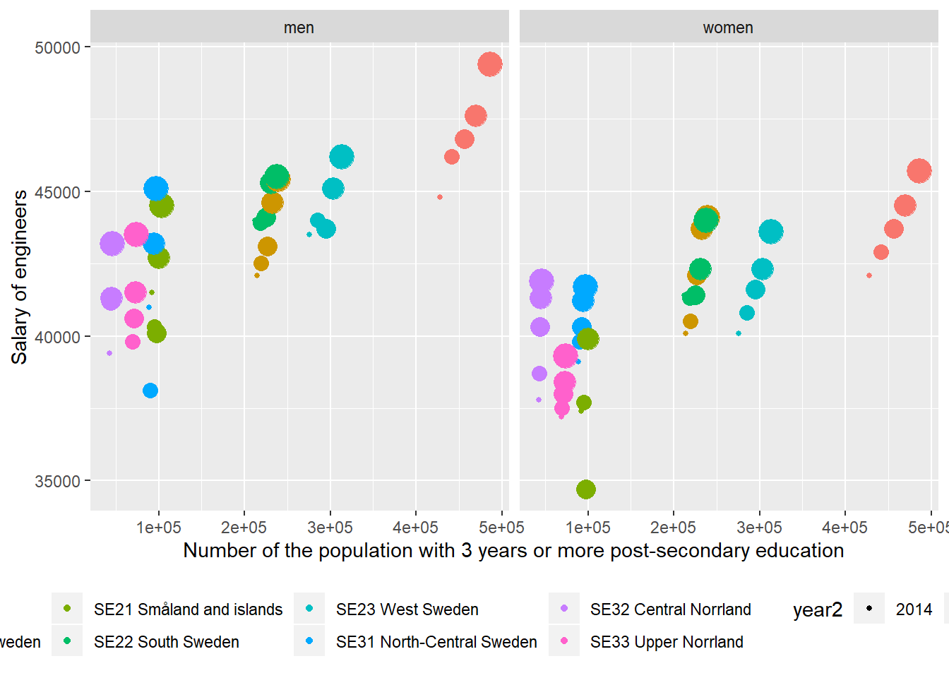
Figure 12.10: The correlation between the salary of engineers and the number of the population who have 3 years or more post-secondary education, but not postgraduate education in the regions (NUTS2), Year 2014 - 2018.
tb <- readfile("000000CG_10.csv")
tb <- readfile("000000CD_10.csv") %>%
  left_join(tb, by = c("region", "year", "sex")) %>%
  group_by (`region`, year) %>%
  mutate (perc_women = as.numeric (sub ("%", "", perc_women (salary.x)))) %>%
  mutate (perc_salary = as.numeric (sub ("%", "", perc_sal (salary.y)))) %>%
  mutate (sum_ing = sum(salary.x))
readfile("UF0506A1_1.csv") %>%
  group_by(`level of education`, region, year, sex) %>%
  mutate(utbregno = sum(salary)) %>%
  group_by(region, year, sex) %>% mutate(perc_edu = utbregno / sum(utbregno)) %>%
  group_by(`level of education`, region, year) %>%
  mutate (sum_edu = sum(utbregno)) %>%
  filter (`level of education` == "post-secondary education 3 years or more (ISCED97 5A)") %>%
  right_join(tb, by = c("region", "year", "sex")) %>%
  mutate (perc_eng = sum_ing / sum_edu) %>%
  ggscatter(x = "sum_edu", y = "salary.y",
  add = "reg.line", conf.int = TRUE,
  cor.coef = TRUE, cor.method = "pearson") +
  facet_grid(. ~ sex) +
  labs(
    x = "Number of the population with 3 years or more post-secondary education",
    y = "Salary of engineers"
  )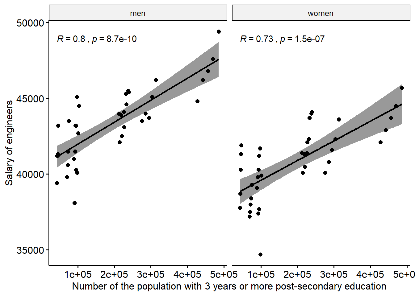
Figure 12.11: The correlation between the salary of engineers and the number of the population who have 3 years or more post-secondary education, but not postgraduate education in the regions (NUTS2), Year 2014 - 2018.
tb <- readfile("000000CG_10.csv")
tb <- readfile("000000CD_10.csv") %>%
  left_join(tb, by = c("region", "year", "sex")) %>%
  group_by (`region`, year) %>%
  mutate (perc_women = as.numeric (sub ("%", "", perc_women (salary.x)))) %>%
  mutate (perc_salary = as.numeric (sub ("%", "", perc_sal (salary.y)))) %>%
  mutate (sum_ing = sum(salary.x))
tb <- readfile("UF0506A1_1.csv") %>%
  group_by(`level of education`, region, year, sex) %>%
  mutate(utbregno = sum(salary)) %>%
  group_by(region, year, sex) %>% mutate(perc_edu = utbregno / sum(utbregno)) %>%
  group_by(region, year) %>% mutate(sum_pop = sum(utbregno)) %>%
  group_by(`level of education`, region, year) %>%
  mutate (sum_edu = sum(utbregno)) %>%
  right_join(tb, by = c("region", "year", "sex")) %>%
  mutate (perc_eng = sum_ing / sum_edu) %>%
  filter (`level of education` == "post-secondary education 3 years or more (ISCED97 5A)")

tb1 <- tb %>%
  ungroup() %>%
  select(utbregno, year2, perc_edu, sum_pop, sum_edu, perc_women, perc_salary, sum_ing, perc_eng, salary.y) %>%
  na.omit()

set.seed(1)

cmodel <- cubist(tb1[, -10], tb1$salary.y)

summary(cmodel)
##
## Call:
## cubist.default(x = tb1[, -10], y = tb1$salary.y)
##
##
## Cubist [Release 2.07 GPL Edition] Sat Nov 09 22:47:29 2019
## ---------------------------------
##
## Target attribute `outcome'
##
## Read 76 cases (10 attributes) from undefined.data
##
## Model:
##
## Rule 1: [76 cases, mean 42077.6, range 34700 to 49400, est err 784.7]
##
## outcome = -1504741.3 + 0.0585 sum_edu - 0.491 sum_ing - 0.027 utbregno
## + 93129 perc_eng + 765 year2 - 17209 perc_edu
##
##
## Evaluation on training data (76 cases):
##
## Average |error| 818.3
## Relative |error| 0.39
## Correlation coefficient 0.90
##
##
## Attribute usage:
## Conds Model
##
## 100% utbregno
## 100% year2
## 100% perc_edu
## 100% sum_edu
## 100% sum_ing
## 100% perc_eng
##
##
## Time: 0.0 secsmodel <- lm(log(salary.y) ~ year2 + perc_edu + sum_edu + sum_ing + perc_eng, data = tb)
summary(model) %>%
tidy() %>%
knitr::kable(
booktabs = TRUE,
caption = 'Salary of engineers and population with 3 years or more post-secondary education')| term | estimate | std.error | statistic | p.value |
|---|---|---|---|---|
| (Intercept) | -28.8586727 | 4.4852648 | -6.434107 | 0.0000000 |
| year2 | 0.0195703 | 0.0022270 | 8.787717 | 0.0000000 |
| perc_edu | -0.6184356 | 0.0682540 | -9.060795 | 0.0000000 |
| sum_edu | 0.0000010 | 0.0000002 | 6.356104 | 0.0000000 |
| sum_ing | -0.0000092 | 0.0000027 | -3.441580 | 0.0009666 |
| perc_eng | 1.5546134 | 0.5363753 | 2.898369 | 0.0049680 |
Anova(model, type=2) %>%
  tidy() %>%
  knitr::kable(
  booktabs = TRUE,
caption = 'Anova report from linear model fit') | term | sumsq | df | statistic | p.value |
|---|---|---|---|---|
| year2 | 0.0565259 | 1 | 77.223967 | 0.0000000 |
| perc_edu | 0.0600936 | 1 | 82.097998 | 0.0000000 |
| sum_edu | 0.0295718 | 1 | 40.400055 | 0.0000000 |
| sum_ing | 0.0086698 | 1 | 11.844473 | 0.0009666 |
| perc_eng | 0.0061490 | 1 | 8.400541 | 0.0049680 |
| Residuals | 0.0527021 | 72 | NA | NA |
12.5 The correlation between the proportion of the population who have 3 years or more post-secondary education and the number of the population who have 3 years or more post-secondary education in the regions, Year 2014 - 2018
tb <- readfile("000000CG_10.csv")
tb <- readfile("000000CD_10.csv") %>%
  left_join(tb, by = c("region", "year", "sex")) %>%
  group_by (`region`, year) %>%
  mutate (perc_women = as.numeric (sub ("%", "", perc_women (salary.x)))) %>%
  mutate (perc_salary = as.numeric (sub ("%", "", perc_sal (salary.y)))) %>%
  mutate (sum_ing = sum(salary.x))
readfile("UF0506A1_1.csv") %>%
  group_by(`level of education`, region, year, sex) %>%
  mutate(utbregno = sum(salary)) %>%
  group_by(region, year, sex) %>% mutate(perc_edu = utbregno / sum(utbregno)) %>%
  group_by(`level of education`, region, year) %>%
  mutate (sum_edu = sum(utbregno)) %>%
  filter (`level of education` == "post-secondary education 3 years or more (ISCED97 5A)") %>%
  right_join(tb, by = c("region", "year", "sex")) %>%
  mutate (perc_eng = sum_ing / sum_edu) %>%
  ggplot(aes(x = perc_edu, y = salary, colour = region, size = year2)) +
  geom_point() +
  theme(legend.position="bottom") +
  facet_grid(. ~ sex) +
  labs(
    x = "Per cent of the population with 3 years or more post-secondary education",
    y = "Number of the population with 3 years or more post-secondary education"
  )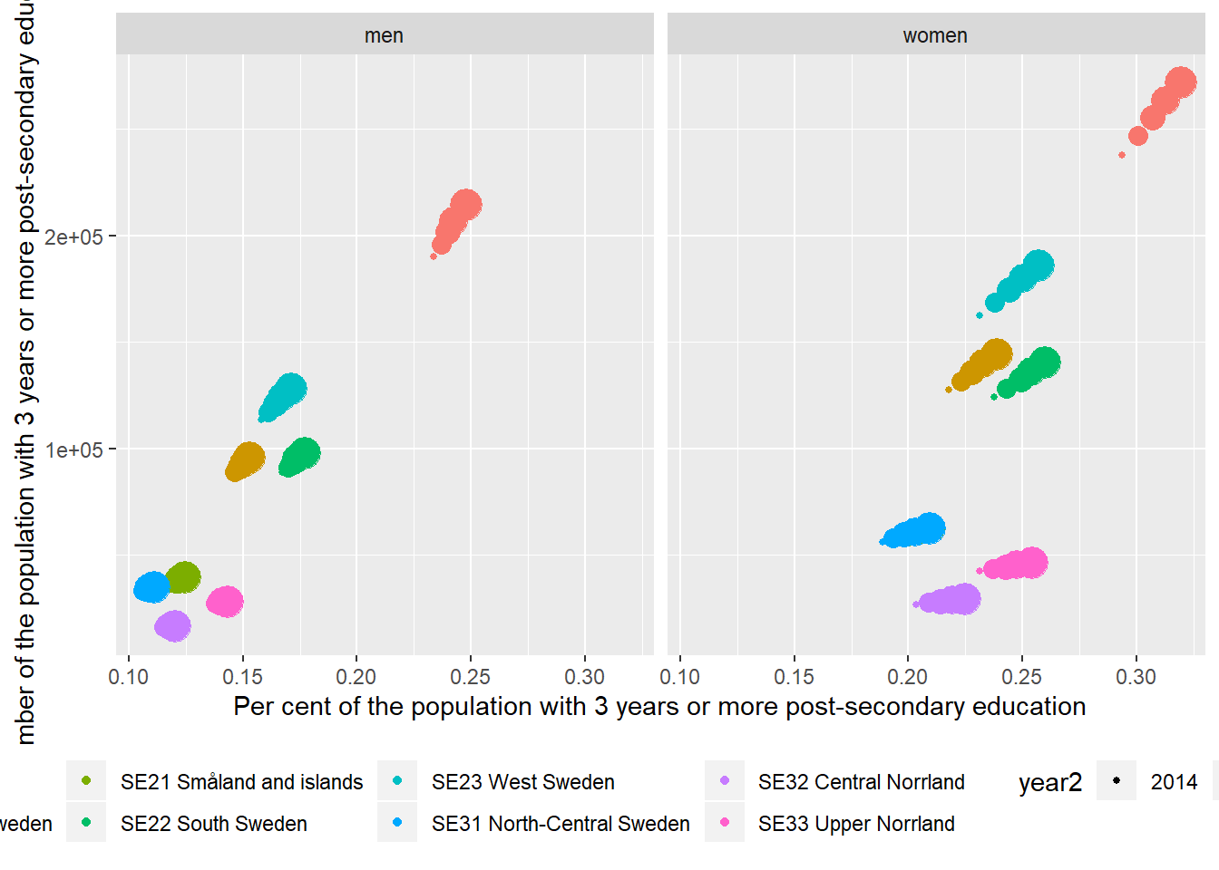
Figure 12.12: The correlation between the proportion of the population who have 3 years or more post-secondary education, but not postgraduate education and the number of the population who have 3 years or more post-secondary education, but not postgraduate education in the regions (NUTS2), Year 2014 - 2018.
12.6 The correlation between the proportion of engineers who are women and the number of the population who have 3 years or more post-secondary education in the region. Year 2003 - 2013
Average basic salary, monthly salary and women´s salary as a percentage of men´s salary by region, sector, occupational group (SSYK 2012) and sex . Year 2003 - 2013 Monthly salaty All sectors 214 Engineering professionals
Average basic salary, monthly salary and women´s salary as a percentage of men´s salary by region, sector, occupational group (SSYK 2012) and sex . Year 2003 - 2013 Number of employees All sectors 214 Engineering professionals
Population 16-74 years of age by region, highest level of education, age and sex. The year 1985 - 2018. total 16-74 years
tb <- readfile("AM0110A2_3.csv")
tb <- readfile("AM0110A4_3.csv") %>%
  left_join(tb, by = c("region", "year", "sex")) %>%
  group_by (`region`, year) %>%
  mutate (perc_women = as.numeric (sub ("%", "", perc_women (salary.x)))) %>%
  mutate (perc_salary = as.numeric (sub ("%", "", perc_sal (salary.y)))) %>%
  mutate (sum_ing = sum(salary.x))
readfile("UF0506A1_1.csv") %>%
  group_by(`level of education`, region, year, sex) %>%
  mutate(utbregno = sum(salary)) %>%
  group_by(region, year, sex) %>% mutate(perc_edu = utbregno / sum(utbregno)) %>%
  group_by(`level of education`, region, year) %>%
  mutate (sum_edu = sum(utbregno)) %>%
  filter (`level of education` == "post-secondary education 3 years or more (ISCED97 5A)") %>%
  right_join(tb, by = c("region", "year", "sex")) %>%
  mutate (perc_eng = sum_ing / sum_edu) %>%
  ggplot(aes(x = sum_edu, y = perc_women, colour = region, size = year2)) +
  geom_point() +
  theme(legend.position="bottom") +
  labs(
    x = "Number of the population with 3 years or more post-secondary education",
    y = "Per cent of engineers who are women"
  )
## Warning: Removed 12 rows containing missing values (geom_point).
Figure 12.13: The correlation between the proportion of engineers who are women and the number of the population who have 3 years or more post-secondary education, but not postgraduate education in the regions (NUTS2), 2003 - 2013.
tb <- readfile("AM0110A2_3.csv")
tb <- readfile("AM0110A4_3.csv") %>%
  left_join(tb, by = c("region", "year", "sex")) %>%
  group_by (`region`, year) %>%
  mutate (perc_women = as.numeric (sub ("%", "", perc_women (salary.x)))) %>%
  mutate (perc_salary = as.numeric (sub ("%", "", perc_sal (salary.y)))) %>%
  mutate (sum_ing = sum(salary.x))
readfile("UF0506A1_1.csv") %>%
  group_by(`level of education`, region, year, sex) %>%
  mutate(utbregno = sum(salary)) %>%
  group_by(region, year, sex) %>% mutate(perc_edu = utbregno / sum(utbregno)) %>%
  group_by(`level of education`, region, year) %>%
  mutate (sum_edu = sum(utbregno)) %>%
  filter (`level of education` == "post-secondary education 3 years or more (ISCED97 5A)") %>%
  right_join(tb, by = c("region", "year", "sex")) %>%
  mutate (perc_eng = sum_ing / sum_edu) %>%
  ggscatter(x = "sum_edu", y = "perc_women",
  add = "reg.line", conf.int = TRUE,
  cor.coef = TRUE, cor.method = "pearson") +
  labs(
    x = "Number of the population with 3 years or more post-secondary education",
    y = "Per cent of engineers who are women"
  )
## Warning: Removed 12 rows containing non-finite values (stat_smooth).## Warning: Removed 12 rows containing non-finite values (stat_cor).## Warning: Removed 12 rows containing missing values (geom_point).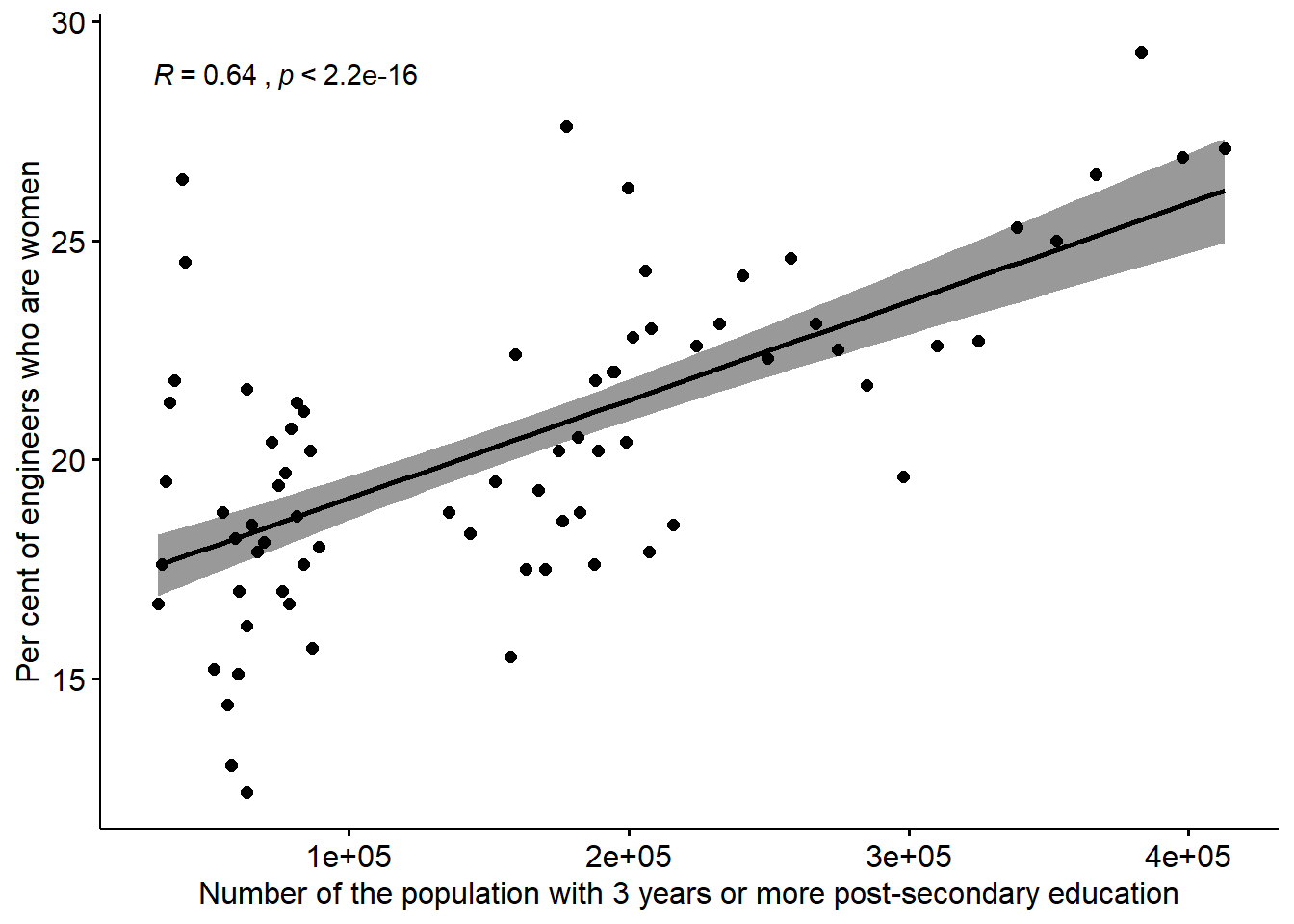
Figure 12.14: The correlation between the proportion of engineers who are women and the number of the population who have 3 years or more post-secondary education, but not postgraduate education in the regions (NUTS2), Year 2003 - 2013.
tb <- readfile("AM0110A2_3.csv")
tb <- readfile("AM0110A4_3.csv") %>%
  left_join(tb, by = c("region", "year", "sex")) %>%
  group_by (`region`, year) %>%
  mutate (perc_women = as.numeric (sub ("%", "", perc_women (salary.x)))) %>%
  mutate (perc_salary = as.numeric (sub ("%", "", perc_sal (salary.y)))) %>%
  mutate (sum_ing = sum(salary.x))
tb <- readfile("UF0506A1_1.csv") %>%
  group_by(`level of education`, region, year, sex) %>%
  mutate(utbregno = sum(salary)) %>%
  group_by(region, year, sex) %>% mutate(perc_edu = utbregno / sum(utbregno)) %>%
  group_by(region, year) %>% mutate(sum_pop = sum(utbregno)) %>%
  group_by(`level of education`, region, year) %>%
  mutate (sum_edu = sum(utbregno)) %>%
  right_join(tb, by = c("region", "year", "sex")) %>%
  mutate (perc_eng = sum_ing / sum_edu) %>%
  filter (`level of education` == "post-secondary education 3 years or more (ISCED97 5A)")

model <- lm(perc_women ~ sum_edu + year2 + log(salary.y), data = tb)

summary(model) %>%
  tidy() %>%
  knitr::kable(
  booktabs = TRUE,
caption = 'Women engineers and population with 3 years or more post-secondary education')| term | estimate | std.error | statistic | p.value |
|---|---|---|---|---|
| (Intercept) | -667.8801009 | 174.6904512 | -3.823220 | 0.0001945 |
| sum_edu | 0.0000181 | 0.0000025 | 7.379324 | 0.0000000 |
| year2 | 0.3172738 | 0.0985096 | 3.220740 | 0.0015763 |
| log(salary.y) | 4.6156447 | 3.0814454 | 1.497883 | 0.1363226 |
Anova(model, type=2) %>%
  tidy() %>%
  knitr::kable(
  booktabs = TRUE,
caption = 'Anova report from linear model fit') | term | sumsq | df | statistic | p.value |
|---|---|---|---|---|
| sum_edu | 304.71404 | 1 | 54.454420 | 0.0000000 |
| year2 | 58.04577 | 1 | 10.373164 | 0.0015763 |
| log(salary.y) | 12.55495 | 1 | 2.243654 | 0.1363226 |
| Residuals | 816.98142 | 146 | NA | NA |
12.7 The correlation between the number of engineers and the number of the population who have 3 years or more post-secondary education in the regions, Year 2003 - 2013.
tb <- readfile("AM0110A2_3.csv")
tb <- readfile("AM0110A4_3.csv") %>%
  left_join(tb, by = c("region", "year", "sex")) %>%
  group_by (`region`, year) %>%
  mutate (perc_women = as.numeric (sub ("%", "", perc_women (salary.x)))) %>%
  mutate (perc_salary = as.numeric (sub ("%", "", perc_sal (salary.y)))) %>%
  mutate (sum_ing = sum(salary.x))
readfile("UF0506A1_1.csv") %>%
  group_by(`level of education`, region, year, sex) %>%
  mutate(utbregno = sum(salary)) %>%
  group_by(region, year, sex) %>% mutate(perc_edu = utbregno / sum(utbregno)) %>%
  group_by(`level of education`, region, year) %>%
  mutate (sum_edu = sum(utbregno)) %>%
  filter (`level of education` == "post-secondary education 3 years or more (ISCED97 5A)") %>%
  right_join(tb, by = c("region", "year", "sex")) %>%
  mutate (perc_eng = sum_ing / sum_edu) %>%
  ggplot(aes(x = sum_edu, y = sum_ing, colour = region, size = year2)) +
  geom_point() +
  theme(legend.position="bottom") +
  labs(
    x = "Number of the population with 3 years or more post-secondary education",
    y = "Number of the population who are engineers"
  )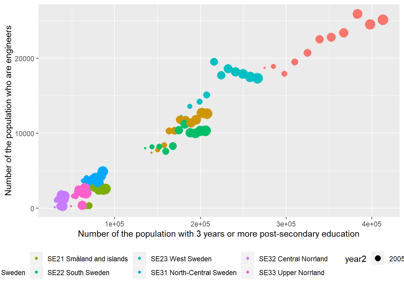
Figure 12.15: The correlation between the number of engineers and the number of the population who have 3 years or more post-secondary education, but not postgraduate education in the regions (NUTS2), Year 2003 - 2013.
tb <- readfile("AM0110A2_3.csv")
tb <- readfile("AM0110A4_3.csv") %>%
  left_join(tb, by = c("region", "year", "sex")) %>%
  group_by (`region`, year) %>%
  mutate (perc_women = as.numeric (sub ("%", "", perc_women (salary.x)))) %>%
  mutate (perc_salary = as.numeric (sub ("%", "", perc_sal (salary.y)))) %>%
  mutate (sum_ing = sum(salary.x))
readfile("UF0506A1_1.csv") %>%
  group_by(`level of education`, region, year, sex) %>%
  mutate(utbregno = sum(salary)) %>%
  group_by(region, year, sex) %>% mutate(perc_edu = utbregno / sum(utbregno)) %>%
  group_by(`level of education`, region, year) %>%
  mutate (sum_edu = sum(utbregno)) %>%
  filter (`level of education` == "post-secondary education 3 years or more (ISCED97 5A)") %>%
  right_join(tb, by = c("region", "year", "sex")) %>%
  mutate (perc_eng = sum_ing / sum_edu) %>%
  ggscatter(x = "sum_edu", y = "sum_ing",
  add = "reg.line", conf.int = TRUE,
  cor.coef = TRUE, cor.method = "pearson") +
  labs(
    x = "Number of the population with 3 years or more post-secondary education",
    y = "Number of the population who are engineers"
  )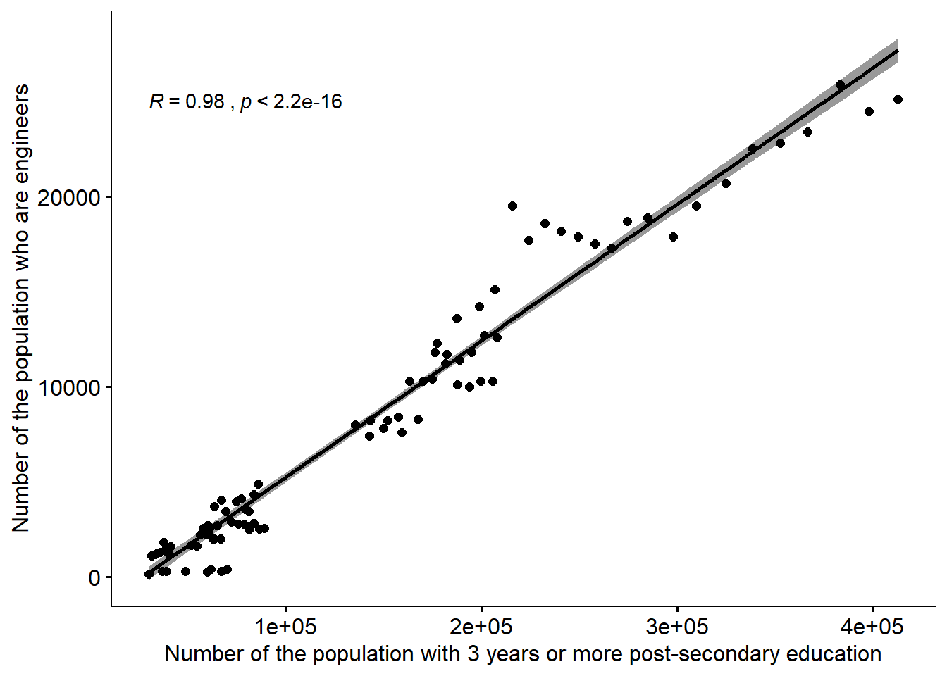
Figure 12.16: The correlation between the number of engineers and the number of the population who have 3 years or more post-secondary education, but not postgraduate education in the regions (NUTS2), Year 2003 - 2013.
tb <- readfile("AM0110A2_3.csv")
tb <- readfile("AM0110A4_3.csv") %>%
  left_join(tb, by = c("region", "year", "sex")) %>%
  group_by (`region`, year) %>%
  mutate (perc_women = as.numeric (sub ("%", "", perc_women (salary.x)))) %>%
  mutate (perc_salary = as.numeric (sub ("%", "", perc_sal (salary.y)))) %>%
  mutate (sum_ing = sum(salary.x))
tb <- readfile("UF0506A1_1.csv") %>%
  group_by(`level of education`, region, year, sex) %>%
  mutate(utbregno = sum(salary)) %>%
  group_by(region, year, sex) %>% mutate(perc_edu = utbregno / sum(utbregno)) %>%
  group_by(region, year) %>% mutate(sum_pop = sum(utbregno)) %>%
  group_by(`level of education`, region, year) %>%
  mutate (sum_edu = sum(utbregno)) %>%
  right_join(tb, by = c("region", "year", "sex")) %>%
  mutate (perc_eng = sum_ing / sum_edu) %>%
  filter (`level of education` == "post-secondary education 3 years or more (ISCED97 5A)")

model <- lm(sum_edu ~ year2 + log(salary.y) * sum_pop, data = tb)

summary(model) %>%
  tidy() %>%
  knitr::kable(
  booktabs = TRUE,
caption = 'Population with 3 years or more post-secondary education and number of population')| term | estimate | std.error | statistic | p.value |
|---|---|---|---|---|
| (Intercept) | 1.267390e+06 | 1.745676e+06 | 0.7260168 | 0.4689094 |
| year2 | 1.147657e+02 | 9.712605e+02 | 0.1181616 | 0.9060907 |
| log(salary.y) | -1.463272e+05 | 4.449966e+04 | -3.2882775 | 0.0012441 |
| sum_pop | -3.221561e+00 | 4.014156e-01 | -8.0254995 | 0.0000000 |
| log(salary.y):sum_pop | 3.274354e-01 | 3.833540e-02 | 8.5413335 | 0.0000000 |
Anova(model, type=2) %>%
  tidy() %>%
  knitr::kable(
  booktabs = TRUE,
caption = 'Anova report from linear model fit') | term | sumsq | df | statistic | p.value |
|---|---|---|---|---|
| year2 | 8075342 | 1 | 0.0139622 | 0.9060907 |
| log(salary.y) | 15636315939 | 1 | 27.0349810 | 0.0000006 |
| sum_pop | 863975869744 | 1 | 1493.8027150 | 0.0000000 |
| log(salary.y):sum_pop | 42194876760 | 1 | 72.9543772 | 0.0000000 |
| Residuals | 90804635841 | 157 | NA | NA |
12.8 The correlation between the number of engineers and the proportion of engineers who are women in the regions, Year 2003 - 2013
tb <- readfile("AM0110A2_3.csv")
tb <- readfile("AM0110A4_3.csv") %>%
  left_join(tb, by = c("region", "year", "sex")) %>%
  group_by (`region`, year) %>%
  mutate (perc_women = as.numeric (sub ("%", "", perc_women (salary.x)))) %>%
  mutate (perc_salary = as.numeric (sub ("%", "", perc_sal (salary.y)))) %>%
  mutate (sum_ing = sum(salary.x))
readfile("UF0506A1_1.csv") %>%
  group_by(`level of education`, region, year, sex) %>%
  group_by(`level of education`, region, year, sex) %>%
  mutate(utbregno = sum(salary)) %>%
  group_by(region, year, sex) %>% mutate(perc_edu = utbregno / sum(utbregno)) %>%
  group_by(`level of education`, region, year) %>%
  mutate (sum_edu = sum(utbregno)) %>%
  filter (`level of education` == "post-secondary education 3 years or more (ISCED97 5A)") %>%
  right_join(tb, by = c("region", "year", "sex")) %>%
  mutate (perc_eng = sum_ing / sum_edu) %>%
  ggplot(aes(x = perc_women, y = sum_ing, colour = region, size = year2)) +
  geom_point() +
  theme(legend.position="bottom") +
  labs(
    x = "Per cent of engineers who are women",
    y = "Number of the population who are engineers"
  )
## Warning: Removed 12 rows containing missing values (geom_point).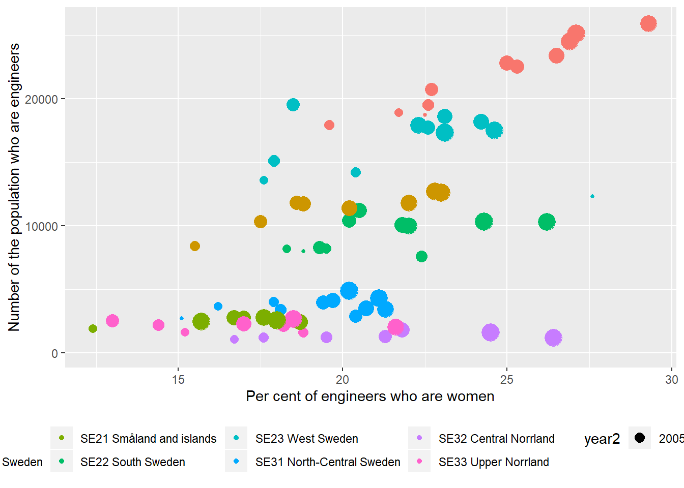
Figure 12.17: The correlation between the number of engineers and the proportion of engineers who are women in the regions (NUTS2), Year 2003 - 2013.
tb <- readfile("AM0110A2_3.csv")
tb <- readfile("AM0110A4_3.csv") %>%
  left_join(tb, by = c("region", "year", "sex")) %>%
  group_by (`region`, year) %>%
  mutate (perc_women = as.numeric (sub ("%", "", perc_women (salary.x)))) %>%
  mutate (perc_salary = as.numeric (sub ("%", "", perc_sal (salary.y)))) %>%
  mutate (sum_ing = sum(salary.x))
readfile("UF0506A1_1.csv") %>%
  group_by(`level of education`, region, year, sex) %>%
  group_by(`level of education`, region, year, sex) %>%
  mutate(utbregno = sum(salary)) %>%
  group_by(region, year, sex) %>% mutate(perc_edu = utbregno / sum(utbregno)) %>%
  group_by(`level of education`, region, year) %>%
  mutate (sum_edu = sum(utbregno)) %>%
  filter (`level of education` == "post-secondary education 3 years or more (ISCED97 5A)") %>%
  right_join(tb, by = c("region", "year", "sex")) %>%
  mutate (perc_eng = sum_ing / sum_edu) %>%
  ggscatter(x = "perc_women", y = "sum_ing",
  add = "reg.line", conf.int = TRUE,
  cor.coef = TRUE, cor.method = "pearson") +
  labs(
    x = "Per cent of engineers who are women",
    y = "Number of the population who are engineers"
  )
## Warning: Removed 12 rows containing non-finite values (stat_smooth).## Warning: Removed 12 rows containing non-finite values (stat_cor).## Warning: Removed 12 rows containing missing values (geom_point).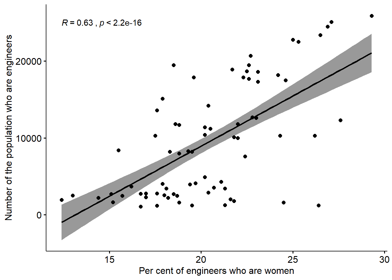
Figure 12.18: The correlation between the number of engineers and the proportion of engineers who are women in the regions (NUTS2), Year 2003 - 2013.
tb <- readfile("AM0110A2_3.csv")
tb <- readfile("AM0110A4_3.csv") %>%
  left_join(tb, by = c("region", "year", "sex")) %>%
  group_by (`region`, year) %>%
  mutate (perc_women = as.numeric (sub ("%", "", perc_women (salary.x)))) %>%
  mutate (perc_salary = as.numeric (sub ("%", "", perc_sal (salary.y)))) %>%
  mutate (sum_ing = sum(salary.x))
tb <- readfile("UF0506A1_1.csv") %>%
  group_by(`level of education`, region, year, sex) %>%
  mutate(utbregno = sum(salary)) %>%
  group_by(region, year, sex) %>% mutate(perc_edu = utbregno / sum(utbregno)) %>%
  group_by(region, year) %>% mutate(sum_pop = sum(utbregno)) %>%
  group_by(`level of education`, region, year) %>%
  mutate (sum_edu = sum(utbregno)) %>%
  right_join(tb, by = c("region", "year", "sex")) %>%
  mutate (perc_eng = sum_ing / sum_edu) %>%
  filter (`level of education` == "post-secondary education 3 years or more (ISCED97 5A)")

model <- lm(sum_ing ~ year2 + log(salary.y) * sum_pop * perc_women, data = tb)

summary(model) %>%
  tidy() %>%
  knitr::kable(
  booktabs = TRUE,
caption = 'Engineers and per cent of engineers who are women')| term | estimate | std.error | statistic | p.value |
|---|---|---|---|---|
| (Intercept) | 3.317429e+05 | 1.975462e+05 | 1.6793176 | 0.0953048 |
| year2 | -1.936866e+02 | 6.830468e+01 | -2.8356265 | 0.0052469 |
| log(salary.y) | 5.175619e+03 | 1.587614e+04 | 0.3259997 | 0.7449079 |
| sum_pop | 1.704584e-01 | 1.735824e-01 | 0.9820029 | 0.3277804 |
| perc_women | 2.164406e+03 | 8.400848e+03 | 0.2576413 | 0.7970594 |
| log(salary.y):sum_pop | -1.568240e-02 | 1.661170e-02 | -0.9440625 | 0.3467526 |
| log(salary.y):perc_women | -2.103752e+02 | 8.024072e+02 | -0.2621801 | 0.7935652 |
| sum_pop:perc_women | -9.808600e-03 | 7.946800e-03 | -1.2342769 | 0.2191529 |
| log(salary.y):sum_pop:perc_women | 9.736000e-04 | 7.581000e-04 | 1.2842003 | 0.2011780 |
Anova(model, type=2) %>%
  tidy() %>%
  knitr::kable(
  booktabs = TRUE,
caption = 'Anova report from linear model fit') | term | sumsq | df | statistic | p.value |
|---|---|---|---|---|
| year2 | 20082665 | 1 | 8.040778 | 0.0052469 |
| log(salary.y) | 24237236 | 1 | 9.704202 | 0.0022277 |
| sum_pop | 3210584661 | 1 | 1285.466737 | 0.0000000 |
| perc_women | 121504617 | 2 | 24.324252 | 0.0000000 |
| log(salary.y):sum_pop | 3146828 | 1 | 1.259939 | 0.2635703 |
| log(salary.y):perc_women | 8443149 | 1 | 3.380502 | 0.0680760 |
| sum_pop:perc_women | 28304085 | 1 | 11.332503 | 0.0009817 |
| log(salary.y):sum_pop:perc_women | 4118972 | 1 | 1.649170 | 0.2011780 |
| Residuals | 352161922 | 141 | NA | NA |
12.9 The correlation between the salary of engineers and the number of the population who have 3 years or more post-secondary education in the regions, Year 2003 - 2013
tb <- readfile("AM0110A2_3.csv")
tb <- readfile("AM0110A4_3.csv") %>%
  left_join(tb, by = c("region", "year", "sex")) %>%
  group_by (`region`, year) %>%
  mutate (perc_women = as.numeric (sub ("%", "", perc_women (salary.x)))) %>%
  mutate (perc_salary = as.numeric (sub ("%", "", perc_sal (salary.y)))) %>%
  mutate (sum_ing = sum(salary.x))
readfile("UF0506A1_1.csv") %>%
  group_by(`level of education`, region, year, sex) %>%
  mutate(utbregno = sum(salary)) %>%
  group_by(region, year, sex) %>% mutate(perc_edu = utbregno / sum(utbregno)) %>%
  group_by(`level of education`, region, year) %>%
  mutate (sum_edu = sum(utbregno)) %>%
  filter (`level of education` == "post-secondary education 3 years or more (ISCED97 5A)") %>%
  right_join(tb, by = c("region", "year", "sex")) %>%
  mutate (perc_eng = sum_ing / sum_edu) %>%
  ggplot(aes(x = sum_edu, y = salary.y, colour = region, size = year2)) +
  geom_point() +
  theme(legend.position="bottom") +
  facet_grid(. ~ sex) +
  labs(
    x = "Number of the population with 3 years or more post-secondary education",
    y = "Salary of engineers"
  )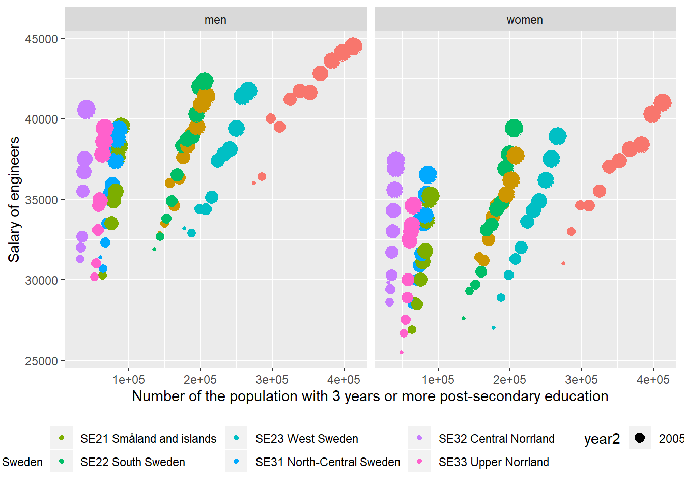
Figure 12.19: The correlation between the salary of engineers and the number of the population who have 3 years or more post-secondary education, but not postgraduate education in the regions (NUTS2), Year 2003 - 2013.
tb <- readfile("AM0110A2_3.csv")
tb <- readfile("AM0110A4_3.csv") %>%
  left_join(tb, by = c("region", "year", "sex")) %>%
  group_by (`region`, year) %>%
  mutate (perc_women = as.numeric (sub ("%", "", perc_women (salary.x)))) %>%
  mutate (perc_salary = as.numeric (sub ("%", "", perc_sal (salary.y)))) %>%
  mutate (sum_ing = sum(salary.x))
readfile("UF0506A1_1.csv") %>%
  group_by(`level of education`, region, year, sex) %>%
  mutate(utbregno = sum(salary)) %>%
  group_by(region, year, sex) %>% mutate(perc_edu = utbregno / sum(utbregno)) %>%
  group_by(`level of education`, region, year) %>%
  mutate (sum_edu = sum(utbregno)) %>%
  filter (`level of education` == "post-secondary education 3 years or more (ISCED97 5A)") %>%
  right_join(tb, by = c("region", "year", "sex")) %>%
  mutate (perc_eng = sum_ing / sum_edu) %>%
  ggscatter(x = "sum_edu", y = "salary.y",
  add = "reg.line", conf.int = TRUE,
  cor.coef = TRUE, cor.method = "pearson") +
  facet_grid(. ~ sex) +
  labs(
    x = "Number of the population with 3 years or more post-secondary education",
    y = "Salary of engineers"
  )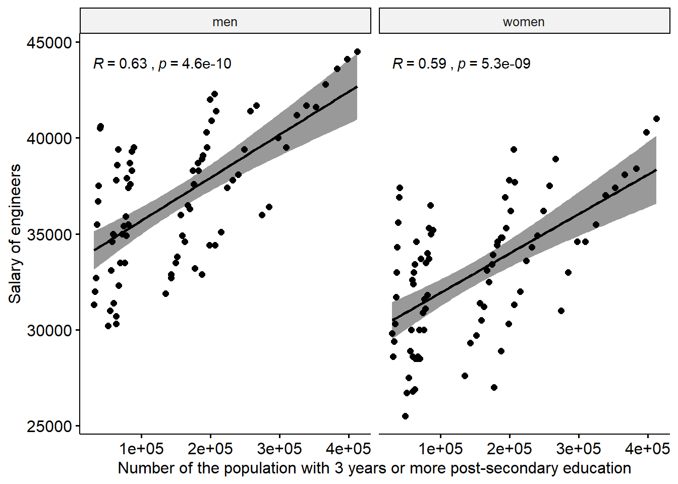
Figure 12.20: The correlation between the salary of engineers and the number of the population who have 3 years or more post-secondary education, but not postgraduate education in the regions (NUTS2), Year 2003 - 2013.
tb <- readfile("AM0110A2_3.csv")
tb <- readfile("AM0110A4_3.csv") %>%
  left_join(tb, by = c("region", "year", "sex")) %>%
  group_by (`region`, year) %>%
  mutate (perc_women = as.numeric (sub ("%", "", perc_women (salary.x)))) %>%
  mutate (perc_salary = as.numeric (sub ("%", "", perc_sal (salary.y)))) %>%
  mutate (sum_ing = sum(salary.x))
tb <- readfile("UF0506A1_1.csv") %>%
  group_by(`level of education`, region, year, sex) %>%
  mutate(utbregno = sum(salary)) %>%
  group_by(region, year, sex) %>% mutate(perc_edu = utbregno / sum(utbregno)) %>%
  group_by(region, year) %>% mutate(sum_pop = sum(utbregno)) %>%
  group_by(`level of education`, region, year) %>%
  mutate (sum_edu = sum(utbregno)) %>%
  right_join(tb, by = c("region", "year", "sex")) %>%
  mutate (perc_eng = sum_ing / sum_edu) %>%
  filter (`level of education` == "post-secondary education 3 years or more (ISCED97 5A)")

tb1 <- tb %>%
  ungroup() %>%
  select(utbregno, year2, perc_edu, sum_pop, sum_edu, perc_women, perc_salary, sum_ing, perc_eng, salary.y) %>%
  na.omit()

set.seed(1)

cmodel <- cubist(tb1[, -10], tb1$salary.y)

summary(cmodel)
##
## Call:
## cubist.default(x = tb1[, -10], y = tb1$salary.y)
##
##
## Cubist [Release 2.07 GPL Edition] Sat Nov 09 22:47:35 2019
## ---------------------------------
##
## Target attribute `outcome'
##
## Read 150 cases (10 attributes) from undefined.data
##
## Model:
##
## Rule 1: [150 cases, mean 35084.0, range 26700 to 44500, est err 938.8]
##
## outcome = -1489479.7 + 0.1162 sum_edu - 0.0929 utbregno - 0.412 sum_ing
## - 0.00608 sum_pop + 755 year2 - 24080 perc_edu
## + 61927 perc_eng + 112 perc_women + 57 perc_salary
##
##
## Evaluation on training data (150 cases):
##
## Average |error| 897.4
## Relative |error| 0.28
## Correlation coefficient 0.96
##
##
## Attribute usage:
## Conds Model
##
## 100% utbregno
## 100% year2
## 100% perc_edu
## 100% sum_pop
## 100% sum_edu
## 100% perc_women
## 100% perc_salary
## 100% sum_ing
## 100% perc_eng
##
##
## Time: 0.0 secsmodel <- lm(log(salary.y) ~ year2 + perc_edu + sum_edu + sum_ing + perc_eng, data = tb)
summary(model) %>%
tidy() %>%
knitr::kable(
booktabs = TRUE,
caption = 'Salary of engineers and population with 3 years or more post-secondary education')| term | estimate | std.error | statistic | p.value |
|---|---|---|---|---|
| (Intercept) | -45.0262481 | 2.6066108 | -17.2738666 | 0.0000000 |
| year2 | 0.0276718 | 0.0013012 | 21.2656449 | 0.0000000 |
| perc_edu | -1.3416735 | 0.1256641 | -10.6766661 | 0.0000000 |
| sum_edu | 0.0000012 | 0.0000003 | 4.5712949 | 0.0000098 |
| sum_ing | -0.0000039 | 0.0000042 | -0.9245089 | 0.3566493 |
| perc_eng | -0.4289334 | 0.5025827 | -0.8534583 | 0.3947138 |
Anova(model, type=2) %>%
  tidy() %>%
  knitr::kable(
  booktabs = TRUE,
caption = 'Anova report from linear model fit') | term | sumsq | df | statistic | p.value |
|---|---|---|---|---|
| year2 | 1.0810807 | 1 | 452.2276514 | 0.0000000 |
| perc_edu | 0.2725036 | 1 | 113.9911980 | 0.0000000 |
| sum_edu | 0.0499551 | 1 | 20.8967375 | 0.0000098 |
| sum_ing | 0.0020433 | 1 | 0.8547167 | 0.3566493 |
| perc_eng | 0.0017413 | 1 | 0.7283910 | 0.3947138 |
| Residuals | 0.3729285 | 156 | NA | NA |