Chapter 10 SSYK 311
10.1 Average monthly salary, SEK by region
Genomsnittlig grund- och månadslön samt kvinnors lön i procent av mäns lön efter region sektor, yrkesgrupp (SSYK 2012) och kön. År 2014 - 2018 Månadslön Samtliga sektorer 311 Ingenjörer och tekniker Kön totalt 2017
readfile ("000000CG_2.csv") %>%
  left_join(nuts, by = c("region" = "NUTS2")) %>%
  right_join(map_ln_n, by = c("Länskod" = "lnkod_n")) %>%
  ggplot() +
    geom_polygon(mapping = aes(x = ggplot_long, y = ggplot_lat, group = lnkod, fill = relsalary)) +
coord_equal() 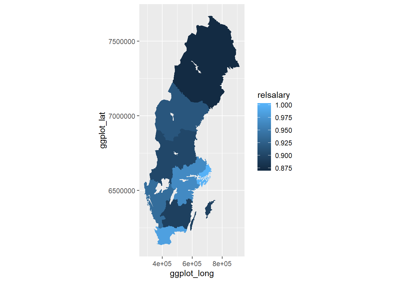
Figure 10.1: Physical and engineering science technicians salaries in the different countys
salary_2017 <- readfile ("000000CG_2.csv") %>%
  left_join(nuts, by = c("region" = "NUTS2"))

readfile ("000000NL_4.csv") %>%
  group_by (`region`, year) %>%
  summarise (perc_women = perc_women (salary)) %>%
  mutate(perc_women_n = as.numeric(sub("%", "", perc_women))) %>%
  mutate(lnkod_n = as.numeric(substr(region, 1,2)))%>%
  right_join(salary_2017, by = c("lnkod_n" = "Länskod")) %>%
  ggscatter(x = "relsalary", y = "perc_women_n",
    add = "reg.line", conf.int = TRUE,
cor.coef = TRUE, cor.method = "pearson") 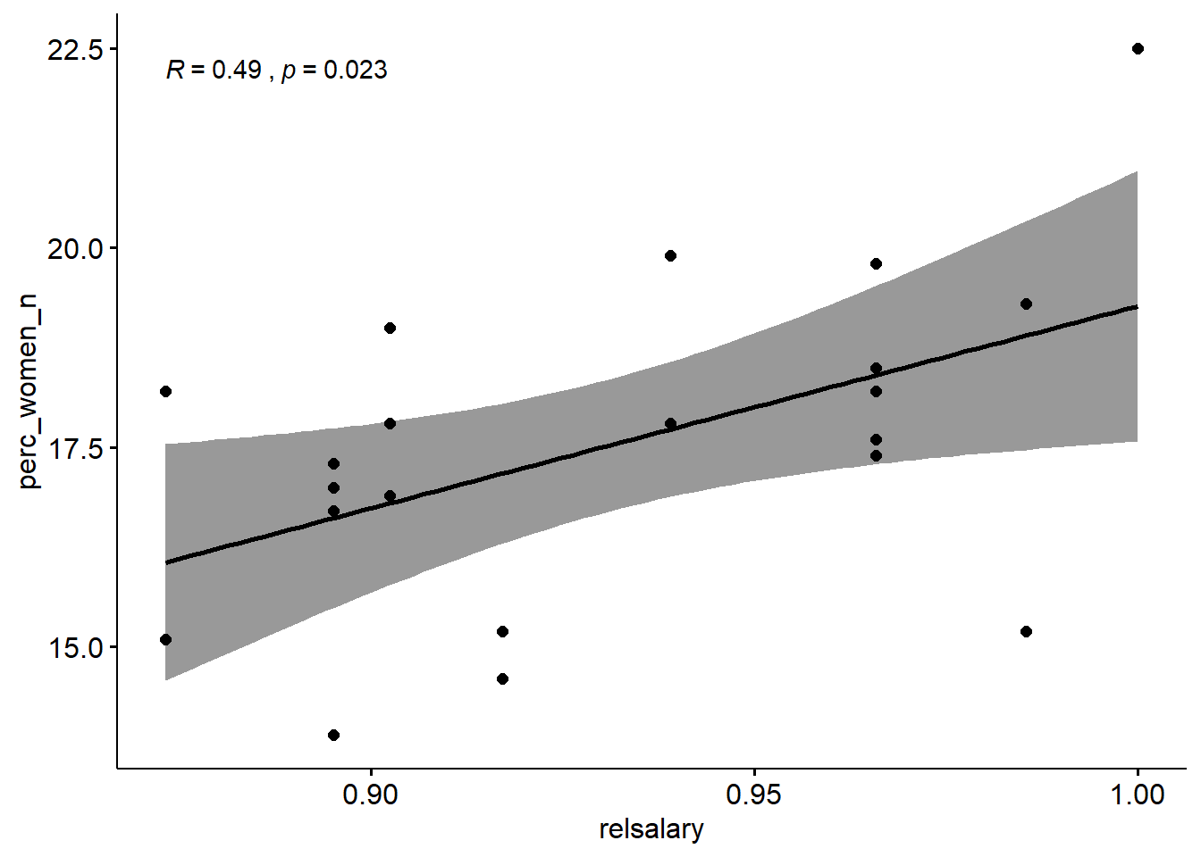
Figure 10.2: The correlation between the proportion of Physical and engineering science technicians who are women and the salaries of engineers in the region.
10.2 Number of men and women in SSYK 311 and the percentage of women in SSYK 311 Year 2014 - 2018
Average basic salary, monthly salary and women´s salary as a percentage of men´s salary by sector, occupational group (SSYK 2012), sex and educational level (SUN). Year 2014 - 2018 Number of employees All sectors 311, Physical and engineering science technicians
readfile("000000CV_4.csv") %>%
  group_by (year) %>%
  mutate (perc_women = as.numeric (sub ("%", "", perc_women (salary)))) %>%
  ggplot(aes(x = year2)) +
  geom_line(mapping = aes(y = salary, colour = sex)) +
  geom_line(mapping = aes(y = perc_women * 2000)) +
  scale_y_continuous(sec.axis = sec_axis(~ . * 0.0005, name = "Percent women [%]"))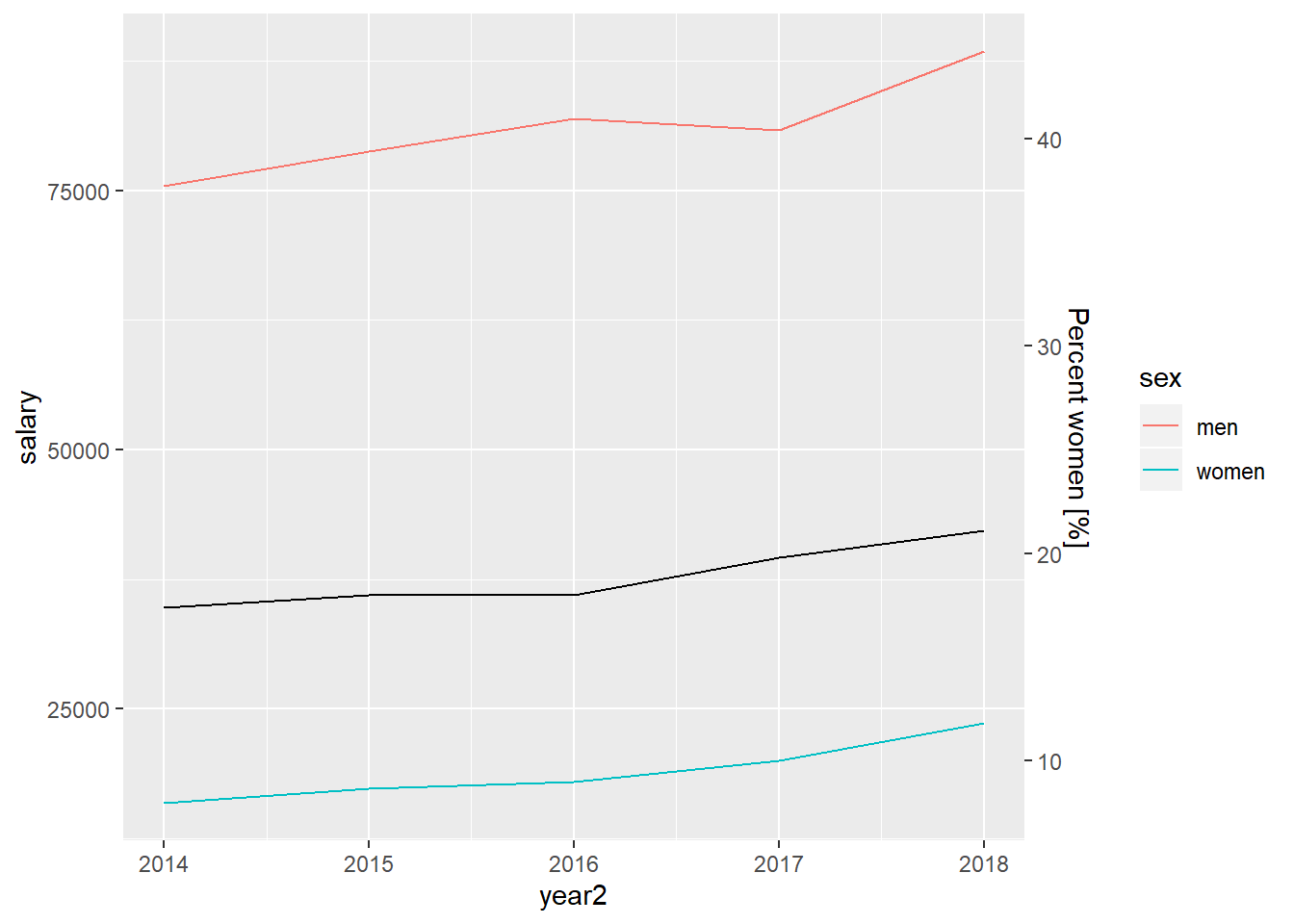
Figure 10.3: Number of men and women in SSYK 311 and the percentage of women in SSYK 311 Year 2014 - 2018
10.3 Number of men and women in SSYK 311 and the percentage of women in SSYK 311 Year 2003 - 2013
Average basic salary, monthly salary and women´s salary as a percentage of men´s salary by sector, occupational group (SSYK), sex and educational level (SUN). Year 2003 - 2013 Number of employees All sectors 311, Physical and engineering science technicians
readfile("AM0110B4_1.csv") %>%
  group_by (year) %>%
  mutate (perc_women = as.numeric (sub ("%", "", perc_women (salary)))) %>%
  ggplot(aes(x = year2)) +
  geom_line(mapping = aes(y = salary, colour = sex)) +
  geom_line(mapping = aes(y = perc_women * 2000)) +
  scale_y_continuous(sec.axis = sec_axis(~ . * 0.0005, name = "Percent women [%]"))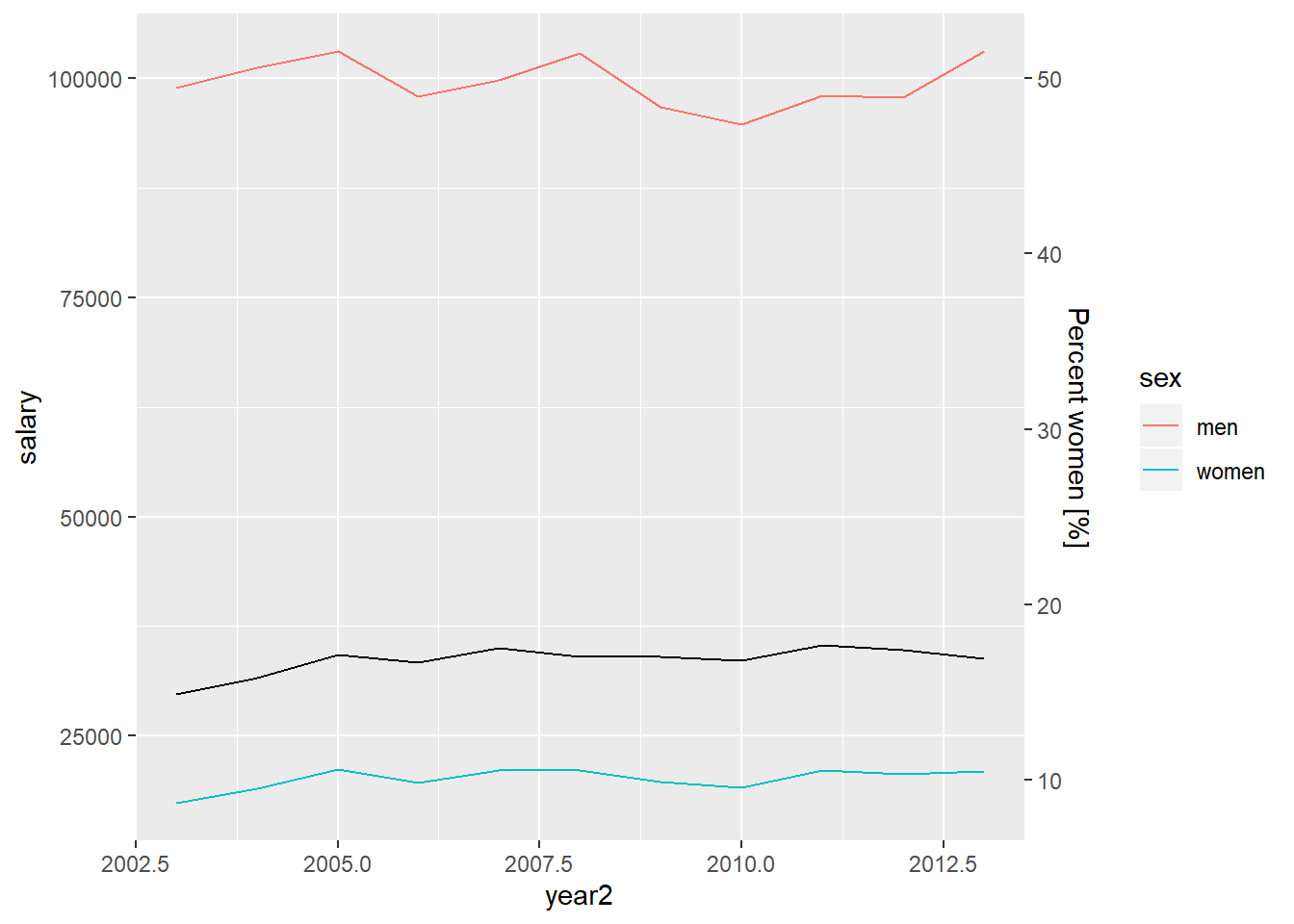
Figure 10.4: Number of men and women in SSYK 311 and the percentage of women in SSYK 311 Year 2003 - 2013
10.4 Age distribution in the different countys
Employees 16-64 years by region of work, occupation (3-digit SSYK 2012), age and sex. Year 2014 - 2017 occupation=SSYK 311, Physical and engineering science technicians
readfile("000000NK_1.csv") %>% filter(year2 == 2017) %>%
  rowwise() %>% mutate(age2 = unlist(lapply(strsplit(substr(age, 1, 5), "-"), strtoi))[1]) %>%
  rowwise() %>% mutate(age3 = unlist(lapply(strsplit(substr(age, 1, 5), "-"), strtoi))[2]) %>%
  ggplot() +
    geom_line(aes(x = (age2 + age3) / 2, y = salary, color = region)) +
    theme(legend.position="bottom") +
    facet_grid(. ~ sex)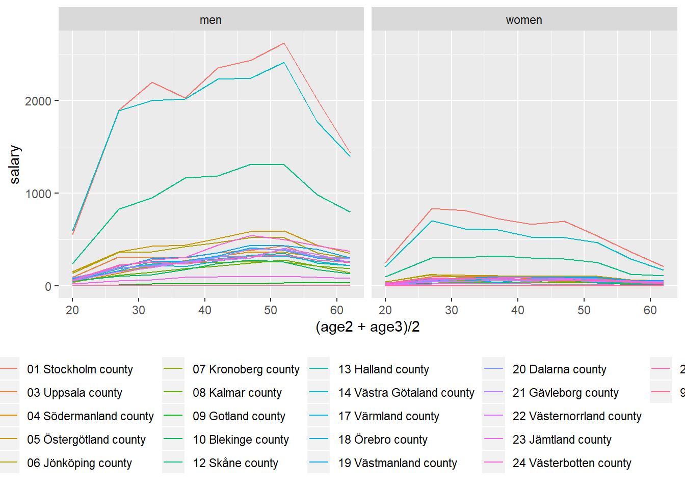
Figure 10.5: The age distribution in the different countys for Physical and engineering science technicians, year 2017
10.5 Sector distribution in the different countys
Employees 16-64 years by region of work, occupation (3-digit SSYK 2012), sector and sex. Year 2014 - 2017 occupation=SSYK 311, Physical and engineering science technicians
readfile("000000RM_2.csv") %>%
  filter(year2 == 2017) %>%
  mutate(lnkod_n = substr(region, 1,2))%>%
  ggplot(aes(x = lnkod_n, y = salary, fill = sector)) +
    geom_col(position = "fill") +
    theme(legend.position="bottom") +
    facet_grid(. ~ sex)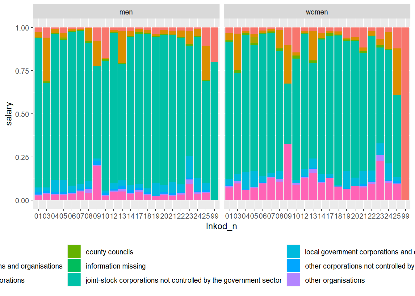
Figure 10.6: The sector distribution in the different countys for Physical and engineering science technicians, year 2017
10.6 Education distribution for engineers
Number of employees by sector, occuptional (SSYK 2012), sex, level of education and year 311, Physical and engineering science technicians All sectors Year 2017
edu <- readfile("000000CV_2.csv")
edu$`level of education` <- as.factor(edu$`level of education`)
edu$`level of education` <- factor(edu$`level of education`, levels(edu$`level of education`)[c(2, 3, 4, 6, 7, 5, 1)])
edu %>%
  filter(year2 == 2017) %>%
  drop_na() %>%
  ggplot(aes(x = `occuptional  (SSYK 2012)`, y = salary, fill = `level of education`)) +
    geom_col(position = "fill") +
    theme(legend.position="bottom") +
facet_grid(. ~ sex) 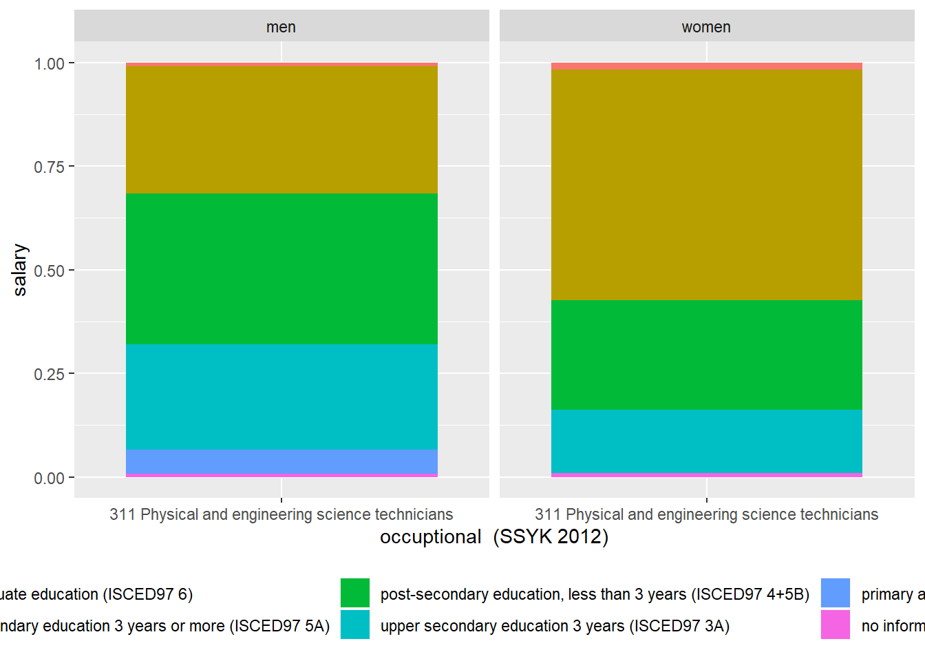
Figure 10.7: The education distribution for Physical and engineering science technicians, year 2017
10.7 SSYK 311, Physical and engineering science technicians, Year 2000 - 2013
Average monthly pay, non-manual workers private sector (SLP) by occupational group (SSYK) age and sex. Year 2000 - 2013 Average monthly pay (total pay), non-manual workers private sector (SLP), SEK by occupational group (SSYK), age, sex and year
tb <- readfile("AM0103A9_3.csv") %>%
  rowwise() %>%
  mutate(age2 = unlist(lapply(strsplit(substr(age, 1, 5), "-"), strtoi))[1]) %>%
  rowwise() %>%
  mutate(age3 = unlist(lapply(strsplit(substr(age, 1, 5), "-"), strtoi))[2]) %>%
  mutate(age4 = (age3 + age2) / 2) %>%
  group_by (`occupational group (SSYK)`, age, sex) %>%
  mutate (grouprelsal = relative_dev (salary))
## Warning: Grouping rowwise data frame strips rowwise naturetb <- tb %>% drop_na()
tb %>%
ggplot () +
geom_point (mapping = aes(x = year2,y = log(salary), colour = age, shape=sex)) 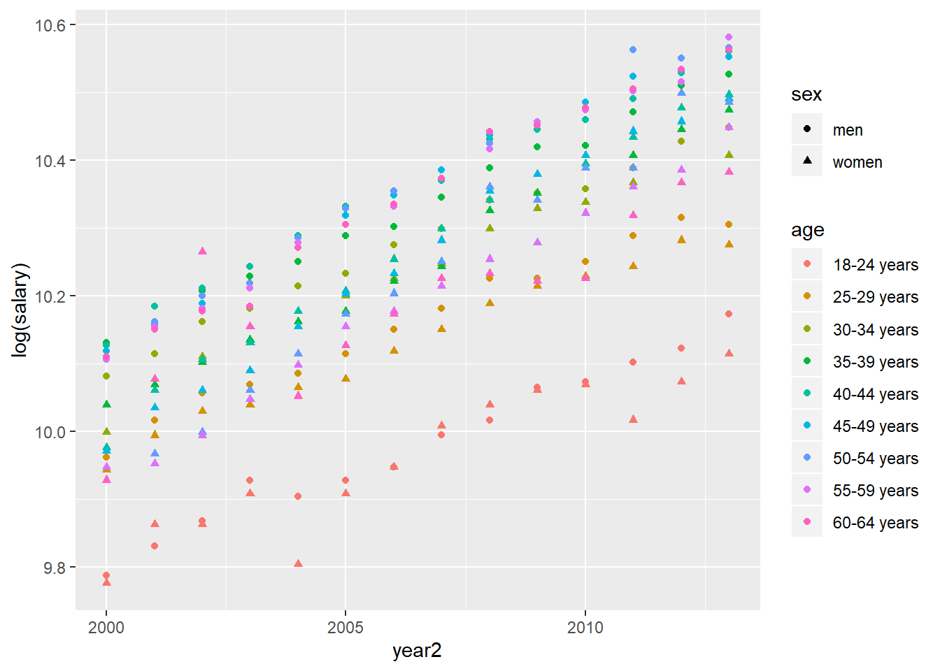
Figure 10.8: SSYK 311, Physical and engineering science technicians, Year 2000 - 2013
tb <- bind_cols(tb, as_tibble(exp(predict(model, tb, interval = "confidence"))))

tb %>%
  ggplot () +
    geom_point (mapping = aes(x = year2,y = log(fit), colour = age, shape=sex))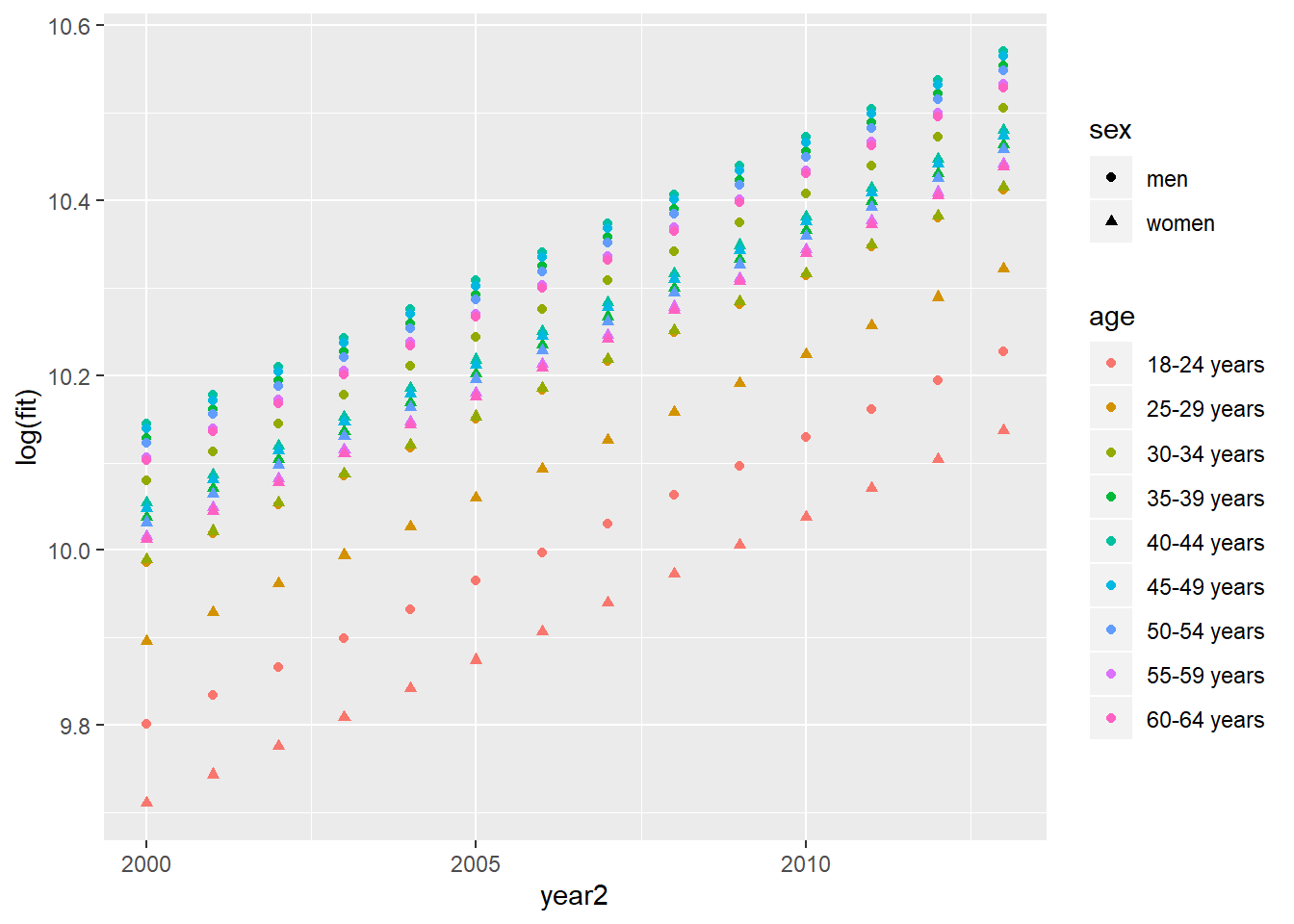
(#fig:311ssyk00-13_2)SSYK, Year 2000 - 2013
summary(model) %>%
  tidy() %>%
  knitr::kable(
  booktabs = TRUE,
caption = 'Summary from linear model fit')| term | estimate | std.error | statistic | p.value |
|---|---|---|---|---|
| (Intercept) | -55.4956164 | 1.3177309 | -42.114529 | 0 |
| year2 | 0.0327817 | 0.0006567 | 49.916675 | 0 |
| sexwomen | -0.0905145 | 0.0052947 | -17.095255 | 0 |
| poly(age4, 3)1 | 1.1571259 | 0.0420255 | 27.533908 | 0 |
| poly(age4, 3)2 | -1.1172447 | 0.0420255 | -26.584930 | 0 |
| poly(age4, 3)3 | 0.4045459 | 0.0420255 | 9.626203 | 0 |
Anova(model, type=2) %>%
  tidy() %>%
  knitr::kable(
  booktabs = TRUE,
caption = 'Anova report from linear model fit') | term | sumsq | df | statistic | p.value |
|---|---|---|---|---|
| year2 | 4.4006501 | 1 | 2491.6745 | 0 |
| sex | 0.5161509 | 1 | 292.2478 | 0 |
| poly(age4, 3) | 2.7508334 | 3 | 519.1795 | 0 |
| Residuals | 0.4344708 | 246 | NA | NA |
10.8 SSYK 311, Physical and engineering science technicians, Year 2014 - 2018
Average monthly pay, non-manual workers private sector (SLP) by occupational group (SSYK 2012) age and sex. Year 2014 - 2018 Average monthly pay (total pay), non-manual workers private sector (SLP), SEK by occupational group (SSYK), age, sex and year
tb <- readfile("00000031_4.csv") %>%
  rowwise() %>%
  mutate(age2 = unlist(lapply(strsplit(substr(age, 1, 5), "-"), strtoi))[1]) %>%
  rowwise() %>%
  mutate(age3 = unlist(lapply(strsplit(substr(age, 1, 5), "-"), strtoi))[2]) %>%
  mutate(age4 = (age3 + age2) / 2) %>%
  group_by (`occuptional  (SSYK 2012)`, age, sex) %>%
  mutate (grouprelsal = relative_dev (salary))
## Warning: Grouping rowwise data frame strips rowwise naturetb <- tb %>% drop_na()
tb %>%
ggplot () +
geom_point (mapping = aes(x = year2,y = log(salary), colour = age, shape=sex)) 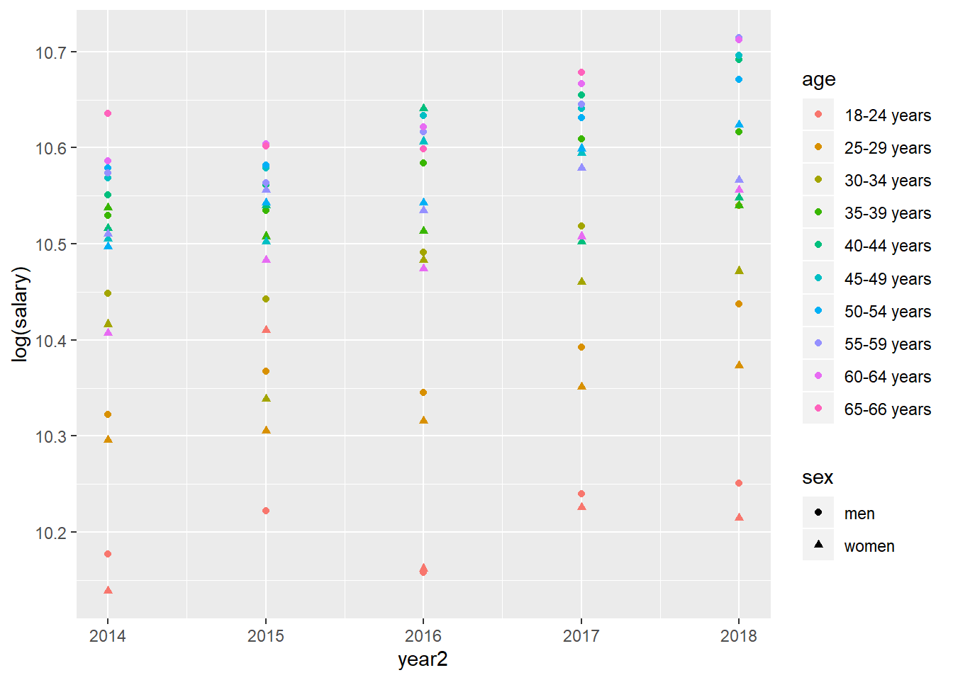
Figure 10.9: SSYK 311, Physical and engineering science technicians, Year 2014 - 2018
model <- lm (log(salary) ~ year2 + sex + poly(age4, 3), data = tb)

tb <- bind_cols(tb, as_tibble(exp(predict(model, tb, interval = "confidence"))))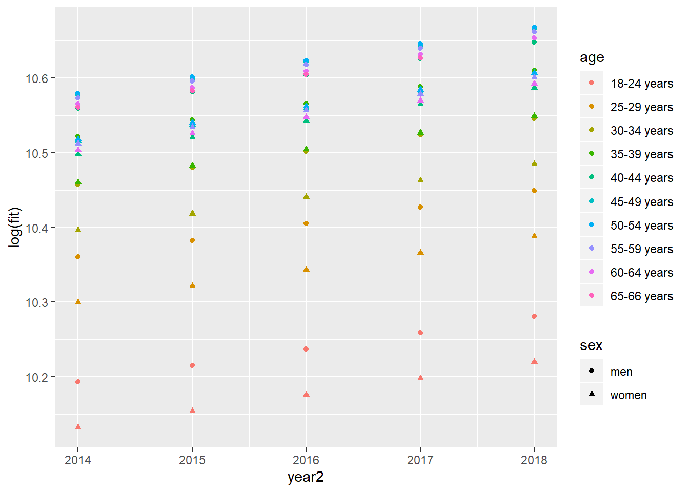
(#fig:311ssyk14-18_2)Model fit, SSYK 311, Physical and engineering science technicians, Year 2014 - 2018
summary(model) %>%
  tidy() %>%
  knitr::kable(
  booktabs = TRUE,
caption = 'Summary from linear model fit')| term | estimate | std.error | statistic | p.value |
|---|---|---|---|---|
| (Intercept) | -33.9739390 | 6.6648565 | -5.097475 | 0.0000020 |
| year2 | 0.0220773 | 0.0033060 | 6.677891 | 0.0000000 |
| sexwomen | -0.0611424 | 0.0093373 | -6.548189 | 0.0000000 |
| poly(age4, 3)1 | 0.9858933 | 0.0446885 | 22.061433 | 0.0000000 |
| poly(age4, 3)2 | -0.6459170 | 0.0446724 | -14.458980 | 0.0000000 |
| poly(age4, 3)3 | 0.1543527 | 0.0447198 | 3.451549 | 0.0008624 |
Anova(model, type=2) %>%
  tidy() %>%
  knitr::kable(
  booktabs = TRUE,
caption = 'Anova report from linear model fit') | term | sumsq | df | statistic | p.value |
|---|---|---|---|---|
| year2 | 0.0884770 | 1 | 44.59423 | 0 |
| sex | 0.0850735 | 1 | 42.87878 | 0 |
| poly(age4, 3) | 1.4109759 | 3 | 237.05355 | 0 |
| Residuals | 0.1726121 | 87 | NA | NA |
10.9 SSYK 311, Physical and engineering science technicians by region, Year 2000 - 2018
Average monthly pay, non-manual workers private sector (SLP) by region, occupational group (SSYK) and sex. Year 2000 - 2013 Average monthly pay (total pay), non-manual workers private sector (SLP) 311, Physical and engineering science technicians
tb <- readfile("AM0103H2_5.csv") %>%
    filter(year2 > 1994) %>%
    group_by (`occupational group (SSYK)`, region, sex) %>%
    mutate (grouprelsal = relative_dev (salary))

model <- lm (log(salary) ~ year2 + region + sex, data = tb)

summary(model) %>%
  tidy() %>%
  knitr::kable(
  booktabs = TRUE,
caption = 'Summary from linear model fit')| term | estimate | std.error | statistic | p.value |
|---|---|---|---|---|
| (Intercept) | -59.8640577 | 0.7758631 | -77.15802 | 0 |
| year2 | 0.0350201 | 0.0003867 | 90.56905 | 0 |
| regionSE12 East-Central Sweden | -0.1057618 | 0.0062348 | -16.96306 | 0 |
| regionSE21 Småland and islands | -0.1584237 | 0.0062348 | -25.40945 | 0 |
| regionSE22 South Sweden | -0.0997065 | 0.0062348 | -15.99185 | 0 |
| regionSE23 West Sweden | -0.0808879 | 0.0062348 | -12.97356 | 0 |
| regionSE31 North-Central Sweden | -0.1292321 | 0.0062348 | -20.72744 | 0 |
| regionSE32 Central Norrland | -0.1702537 | 0.0062348 | -27.30686 | 0 |
| regionSE33 Upper Norrland | -0.1535519 | 0.0062348 | -24.62807 | 0 |
| sexwomen | -0.1088315 | 0.0031174 | -34.91082 | 0 |
Anova(model, type=2) %>%
  tidy() %>%
  knitr::kable(
  booktabs = TRUE,
caption = 'Anova report from linear model fit') | term | sumsq | df | statistic | p.value |
|---|---|---|---|---|
| year2 | 4.4641325 | 1 | 8202.7533 | 0 |
| region | 0.5956647 | 7 | 156.3603 | 0 |
| sex | 0.6632809 | 1 | 1218.7653 | 0 |
| Residuals | 0.1164639 | 214 | NA | NA |
Average monthly pay, non-manual workers private sector (SLP) by region, occupational group (SSYK 2012) and sex. Year 2014 - 2018 Average monthly pay (total pay), non-manual workers private sector (SLP) 311, Physical and engineering science technicians
tb <- readfile("0000002T_2.csv") %>%
    filter(year2 > 1994) %>%
    group_by (`occuptional  (SSYK 2012)`, region, sex) %>%
    mutate (grouprelsal = relative_dev (salary))

model <- lm (log(salary) ~ year2 + region + sex, data = tb)

summary(model) %>%
  tidy() %>%
  knitr::kable(
  booktabs = TRUE,
caption = 'Summary from linear model fit')| term | estimate | std.error | statistic | p.value |
|---|---|---|---|---|
| (Intercept) | -38.2119071 | 5.8520428 | -6.529670 | 0.0000000 |
| year2 | 0.0242250 | 0.0029031 | 8.344477 | 0.0000000 |
| regionSE12 East-Central Sweden | -0.0623028 | 0.0164160 | -3.795259 | 0.0003165 |
| regionSE21 Småland and islands | -0.1353062 | 0.0164160 | -8.242356 | 0.0000000 |
| regionSE22 South Sweden | -0.0496852 | 0.0164160 | -3.026641 | 0.0034903 |
| regionSE23 West Sweden | -0.0695717 | 0.0164160 | -4.238050 | 0.0000695 |
| regionSE31 North-Central Sweden | -0.1103428 | 0.0164160 | -6.721675 | 0.0000000 |
| regionSE32 Central Norrland | -0.0948292 | 0.0168471 | -5.628813 | 0.0000004 |
| regionSE33 Upper Norrland | -0.1371763 | 0.0164160 | -8.356276 | 0.0000000 |
| sexwomen | -0.0773173 | 0.0080931 | -9.553493 | 0.0000000 |
Anova(model, type=2) %>%
  tidy() %>%
  knitr::kable(
  booktabs = TRUE,
caption = 'Anova report from linear model fit') | term | sumsq | df | statistic | p.value |
|---|---|---|---|---|
| year2 | 0.0886793 | 1 | 69.63030 | 0 |
| region | 0.1443745 | 7 | 16.19453 | 0 |
| sex | 0.1162381 | 1 | 91.26922 | 0 |
| Residuals | 0.0866030 | 68 | NA | NA |
10.10 Level of education , SSYK 311, Physical and engineering science technicians
Average basic salary, monthly salary and women´s salary as a percentage of men´s salary by sector, occupational group (SSYK 2012), sex and educational level (SUN). Year 2014 - 2018 Monthly salary 5 non-manual workers private sector 311, Physical and engineering science technicians
tb <- readfile("000000CY_1.csv") %>%
    group_by (`level of education`, sex) %>%
    mutate (grouprelsal = relative_dev (salary))

model <- lm (log(salary) ~ `level of education` + sex + year2, data = tb)

summary(model) %>%
  tidy() %>%
  knitr::kable(
  booktabs = TRUE,
caption = 'Level of education for SSYK 311')| term | estimate | std.error | statistic | p.value |
|---|---|---|---|---|
| (Intercept) | -17.9111596 | 9.1404620 | -1.959546 | 0.0549454 |
level of educationpost-graduate education (ISCED97 6) |
0.1619429 | 0.0270256 | 5.992211 | 0.0000001 |
level of educationpost-secondary education 3 years or more (ISCED97 5A) |
-0.0289399 | 0.0270256 | -1.070834 | 0.2887572 |
level of educationpost-secondary education, less than 3 years (ISCED97 4+5B) |
-0.0833765 | 0.0270256 | -3.085097 | 0.0031371 |
level of educationprimary and secondary education 9-10 years (ISCED97 2) |
-0.2484809 | 0.0270256 | -9.194290 | 0.0000000 |
level of educationprimary and secondary education less than 9 years (ISCED97 1) |
-0.3074331 | 0.0429619 | -7.155943 | 0.0000000 |
level of educationupper secondary education 3 years (ISCED97 3A) |
-0.1793256 | 0.0270256 | -6.635405 | 0.0000000 |
level of educationupper secondary education, 2 years or less (ISCED97 3C) |
-0.1451270 | 0.0275362 | -5.270417 | 0.0000022 |
| sexwomen | -0.1245220 | 0.0130741 | -9.524327 | 0.0000000 |
| year2 | 0.0141833 | 0.0045332 | 3.128745 | 0.0027657 |
Anova(model, type=2) %>%
  tidy() %>%
  knitr::kable(
  booktabs = TRUE,
caption = 'Anova report from linear model fit') | term | sumsq | df | statistic | p.value |
|---|---|---|---|---|
level of education |
1.1652226 | 7 | 62.613589 | 0.0000000 |
| sex | 0.2411631 | 1 | 90.712799 | 0.0000000 |
| year2 | 0.0260245 | 1 | 9.789046 | 0.0027657 |
| Residuals | 0.1515365 | 57 | NA | NA |
10.11 The correlation between the proportion of engineers who are women and the salaries of engineers in the region. Year 2014 - 2018
Average basic salary, monthly salary and women´s salary as a percentage of men´s salary by region, sector, occupational group (SSYK 2012) and sex . Year 2014 - 2018 Number of employees All sectors 311, Physical and engineering science technicians
tb <- readfile("000000CG_11.csv")
tb <- readfile("000000CD_11.csv") %>%
  left_join(tb, by = c("region", "year", "sex")) %>%
  group_by (`region`, year) %>%
  mutate (perc_women = as.numeric (sub ("%", "", perc_women (salary.x))))

model <- lm (log(salary.y) ~ year2.x + perc_women, data = tb)

summary(model) %>%
  tidy() %>%
  knitr::kable(
  booktabs = TRUE,
caption = 'The correlation between the proportion of Physical and engineering science technicians who are women and the salaries of Physical and engineering science technicians in the region. Year 2014 - 2018')| term | estimate | std.error | statistic | p.value |
|---|---|---|---|---|
| (Intercept) | -20.0133859 | 10.7201609 | -1.866892 | 0.0664277 |
| year2.x | 0.0150489 | 0.0053256 | 2.825776 | 0.0062590 |
| perc_women | 0.0102505 | 0.0026313 | 3.895598 | 0.0002340 |
Anova(model, type=2) %>%
  tidy() %>%
  knitr::kable(
  booktabs = TRUE,
caption = 'Anova report from linear model fit') | term | sumsq | df | statistic | p.value |
|---|---|---|---|---|
| year2.x | 0.0262559 | 1 | 7.985011 | 0.006259 |
| perc_women | 0.0498999 | 1 | 15.175685 | 0.000234 |
| Residuals | 0.2137295 | 65 | NA | NA |
10.12 The correlation between the proportion of engineers who are women and the salaries of engineers in the region. Year 2003 - 2013
Average basic salary, monthly salary and women´s salary as a percentage of men´s salary by region, sector, occupational group (SSYK 2012) and sex . Year 2003 - 2013 Number of employees All sectors 311, Physical and engineering science technicians
tb <- readfile("AM0110A2_1.csv")
tb <- readfile("AM0110A4_1.csv") %>%
  left_join(tb, by = c("region", "year", "sex")) %>%
  group_by (`region`, year) %>%
  mutate (perc_women = as.numeric (sub ("%", "", perc_women (salary.x))))

model <- lm (log(salary.y) ~ year2.x + perc_women, data = tb)

summary(model) %>%
  tidy() %>%
  knitr::kable(
  booktabs = TRUE,
caption = 'The correlation between the proportion of Physical and engineering science technicians who are women and the salaries of Physical and engineering science technicians in the region. Year 2003 - 2013')| term | estimate | std.error | statistic | p.value |
|---|---|---|---|---|
| (Intercept) | -52.4842781 | 3.5978522 | -14.587669 | 0 |
| year2.x | 0.0310991 | 0.0017977 | 17.299551 | 0 |
| perc_women | 0.0192601 | 0.0026708 | 7.211263 | 0 |
Anova(model, type=2) %>%
  tidy() %>%
  knitr::kable(
  booktabs = TRUE,
caption = 'Anova report from linear model fit') | term | sumsq | df | statistic | p.value |
|---|---|---|---|---|
| year2.x | 1.4255369 | 1 | 299.27447 | 0 |
| perc_women | 0.2477031 | 1 | 52.00231 | 0 |
| Residuals | 0.7573662 | 159 | NA | NA |
10.13 Animations , SSYK 214, Architects, engineers and related professionals
Approximaton with B-spline
Average monthly pay (total pay), non-manual workers private sector (SLP),
SEK by occuptional group (SSYK), age, sex and year 2000-2013
311, Physical and engineering science technicians
sex=total
readfile("AM0103A9_10.csv") %>% rowwise() %>% mutate(age2 = unlist(lapply(strsplit(substr(age, 1, 5), "-"), strtoi))[1]) %>%
rowwise() %>% mutate(age3 = unlist(lapply(strsplit(substr(age, 1, 5), "-"), strtoi))[2]) %>%
 ggplot(mapping = aes(x = year2 - (age2 + age3) / 2, y = salary)) +
   geom_point() +
   geom_smooth(method = lm, formula = y ~ splines::bs(x, 8), se = FALSE) +
   transition_time(year2) +
   labs(title = "Year: {frame_time}") +
    scale_x_continuous(name = "Year of birth") +
   scale_y_continuous(name = "Salary")
anim_save("311_2000-2013.gif", width = 1000, height = 1000) 
Average monthly pay (total pay), non-manual workers private sector (SLP),
SEK by occuptional (SSYK 2012), age, sex and year 2014-2018
311, Physical and engineering science technicians
sex=total
readfile("00000031_10.csv") %>% rowwise() %>% mutate(age2 = unlist(lapply(strsplit(substr(age, 1, 5), "-"), strtoi))[1]) %>%
rowwise() %>% mutate(age3 = unlist(lapply(strsplit(substr(age, 1, 5), "-"), strtoi))[2]) %>%
 ggplot(mapping = aes(x = year2 - (age2 + age3) / 2, y = salary)) +
   geom_point() +
   geom_smooth(method = lm, formula = y ~ splines::bs(x, 8), se = FALSE) +
   transition_time(year2) +
   labs(title = "Year: {frame_time}") +
    scale_x_continuous(name = "Year of birth") +
   scale_y_continuous(name = "Salary")
anim_save("311_2014-2018.gif", width = 1000, height = 1000) 
Average monthly pay (total pay), non-manual workers private sector (SLP),
SEK by occuptional (SSYK 2012), age, sex and year 2000-2013
311, Physical and engineering science technicians
sex=total
Growth of salaries by age group
csvfile <- readfile("AM0103A9_10.csv") %>%
  rowwise() %>%
  mutate(age2 = unlist(lapply(strsplit(substr(age, 1, 5), "-"), strtoi))[1]) %>%
  rowwise() %>% mutate(age3 = unlist(lapply(strsplit(substr(age, 1, 5), "-"), strtoi))[2])
yearwise <- group_split(csvfile %>% group_by(year2))
ageGroupGrowth = data.frame()
for (i in 1:13){
  temp <- cbind(year = 1999 + i, age = (yearwise[[i]]$age2 + yearwise[[i]]$age3) / 2, growth = yearwise[[i+1]]$relsalary / yearwise[[i]]$relsalary) - 1
  ageGroupGrowth <- rbind(ageGroupGrowth, temp)
}
ageGroupGrowth[, 'age'] <- factor(ageGroupGrowth[, 'age'])
ageGroupGrowth %>%
  ggplot(mapping = aes(x = age, y = growth)) +
  geom_bar(stat = "identity") +
  transition_time(as.numeric(year)) +
  labs(title = "Year: {frame_time}") +
  scale_x_discrete(name = "Age group") +
  scale_y_continuous(name = "Salary increase (%)")
anim_save("311_AgeGroupGrowth2000-2013.gif", width = 1000, height = 1000) 
Average monthly pay (total pay), non-manual workers private sector (SLP),
SEK by occuptional (SSYK 2012), age, sex and year 2000-2013
311, Physical and engineering science technicians
sex=total
Individual salary increase by birthyear, estimated from B-spline approximation
csvfile <- readfile("AM0103A9_10.csv") %>%
  rowwise() %>%
  mutate(age2 = unlist(lapply(strsplit(substr(age, 1, 5), "-"), strtoi))[1]) %>%
  rowwise() %>% mutate(age3 = unlist(lapply(strsplit(substr(age, 1, 5), "-"), strtoi))[2])
indGrowth = data.frame()
for (i in 2000:2012){
  yearfile <- filter(csvfile, year2 == i)
  x = yearfile$year2 - (yearfile$age2 + yearfile$age3) / 2
  model = lm(yearfile$salary ~ splines::bs(x, 8))
  X1 = data.frame(x = unlist(map2( i - 62, i - 22, seq)))
  Y1 = predict(model, X1)
  yearfile <- filter(csvfile, year2 == i + 1)
  x = yearfile$year2 - (yearfile$age2 + yearfile$age3) / 2
  model = lm(yearfile$salary ~ splines::bs(x, 8))
  X2 = data.frame(x = unlist(map2( i + 1 - 62, i + 1 - 22, seq)))
  Y2 = predict(model, X2)
  growth = Y2[1:40] / Y1[2:41]
  temp <- as_tibble(cbind(year = i+1, by=X2[1:40,1], growth=growth))
  indGrowth <- rbind(indGrowth, temp)
}
indGrowth %>%
  ggplot(mapping = aes(x = by, y = growth)) +
  geom_line() +
 transition_time(year) +
  labs(title = "Year: {frame_time}") +
  scale_x_continuous(name = "Year of birth") +
  scale_y_continuous(name = "Salary increase (%)")
anim_save("311_indGrowth2000-2013.gif", width = 1000, height = 1000) 
Average monthly pay (total pay), non-manual workers private sector (SLP),
SEK by occuptional (SSYK 2012), age, sex and year 2000-2013
311, Physical and engineering science technicians
sex=total
Changes in the salary structure part by birthyear, salary structure part is
defined as the derivative of the age / salary function, salary structure
part defines how much the salaries needs to increase each year so that the
structure remains unchanged.
csvfile <- readfile("AM0103A9_10.csv") %>%
  rowwise() %>%
  mutate(age2 = unlist(lapply(strsplit(substr(age, 1, 5), "-"), strtoi))[1]) %>%
  rowwise() %>% mutate(age3 = unlist(lapply(strsplit(substr(age, 1, 5), "-"), strtoi))[2])
salaryStructure = data.frame()
for (i in min(csvfile$year2):max(csvfile$year2)){
  yearfile <- filter(csvfile, year2 == i)
  x = yearfile$year2 - (yearfile$age2 + yearfile$age3) / 2
  model = lm(yearfile$salary ~ splines::bs(x, 8))
  X = data.frame(x = unlist(map2( i - 62, i - 22, seq, length = 100)))
  Y = predict(model, X)
  dX = rowMeans(embed(X$x, 2))
  dY = -diff(Y) / diff(X$x) / Y
  temp <- as_tibble(cbind(year = i, dX = dX, dY = dY))
  salaryStructure <- rbind(salaryStructure, temp)
}
salaryStructure %>%
  ggplot(mapping = aes(x = dX, y = dY)) +
  geom_line() +
  transition_time(year) +
  labs(title = "Year: {frame_time}") +
  scale_x_continuous(name = "Year of birth") +
  scale_y_continuous(name = "Structural increase (%)")
anim_save("311_salaryStructure2000-2013.gif", width = 1000, height = 1000)