Chapter 13 The correlation between the proportion of Physical and engineering science technicians who are women and the number of the population in the region. Year 2014 - 2018
Average basic salary, monthly salary and women´s salary as a percentage of men´s salary by region, sector, occupational group (SSYK 2012) and sex . Year 2014 - 2018 Monthly salaty All sectors 311 Physical and engineering science technicians
Average basic salary, monthly salary and women´s salary as a percentage of men´s salary by region, sector, occupational group (SSYK 2012) and sex . Year 2014 - 2018 Number of employees All sectors 311 Physical and engineering science technicians
Population 16-74 years of age by region, highest level of education, age and sex. Year 1985 - 2018 total 16-74 years
tb <- readfile("000000CG_12.csv")
tb <- readfile("000000CD_12.csv") %>%
  left_join(tb, by = c("region", "year", "sex")) %>%
  drop_na %>%
  group_by (`region`, year) %>%
  mutate (perc_women = as.numeric (sub ("%", "", perc_women (salary.x)))) %>%
  mutate (perc_salary = as.numeric (sub ("%", "", perc_sal (salary.y)))) %>%
  mutate (sum_ing = sum(salary.x))
readfile("UF0506A1_1.csv") %>%
  group_by(`level of education`, region, year, sex) %>%
  mutate(utbregno = sum(salary)) %>%
  group_by(region, year, sex) %>% mutate(perc_edu = utbregno / sum(utbregno)) %>%
  group_by(region, year) %>% mutate(sum_pop = sum(utbregno)) %>%
  group_by(`level of education`, region, year) %>%
  mutate (sum_edu = sum(utbregno)) %>%
  right_join(tb, by = c("region", "year", "sex")) %>%
  mutate (perc_eng = sum_ing / sum_edu) %>%
  ggplot(aes(x = sum_pop, y = perc_women, colour = region, size = year2)) +
  geom_point() +
  theme(legend.position="bottom") +
  labs(
    x = "Number of population",
    y = "Per cent of technicians who are women"
  )
## Warning: Removed 56 rows containing missing values (geom_point).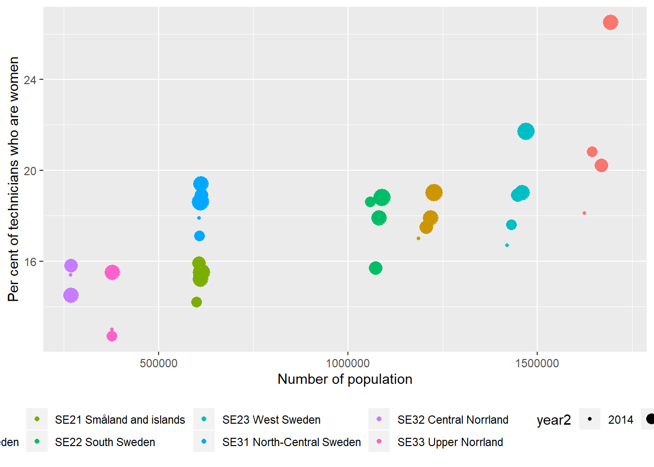
Figure 13.1: The correlation between the proportion of Physical and engineering science technicians who are women and the number of the population in the regions (NUTS2), Year 2014 - 2018.
tb <- readfile("000000CG_12.csv")
tb <- readfile("000000CD_12.csv") %>%
  left_join(tb, by = c("region", "year", "sex")) %>%
  drop_na %>%
  group_by (`region`, year) %>%
  mutate (perc_women = as.numeric (sub ("%", "", perc_women (salary.x)))) %>%
  mutate (perc_salary = as.numeric (sub ("%", "", perc_sal (salary.y)))) %>%
  mutate (sum_ing = sum(salary.x))
readfile("UF0506A1_1.csv") %>%
  group_by(`level of education`, region, year, sex) %>%
  mutate(utbregno = sum(salary)) %>%
  group_by(region, year, sex) %>% mutate(perc_edu = utbregno / sum(utbregno)) %>%
  group_by(region, year) %>% mutate(sum_pop = sum(utbregno)) %>%
  group_by(`level of education`, region, year) %>%
  mutate (sum_edu = sum(utbregno)) %>%
  right_join(tb, by = c("region", "year", "sex")) %>%
  mutate (perc_eng = sum_ing / sum_edu) %>%
  ggscatter(x = "sum_pop", y = "perc_women",
  add = "reg.line", conf.int = TRUE,
  cor.coef = TRUE, cor.method = "pearson") +
  labs(
    x = "Number of population",
    y = "Per cent of technicians who are women"
  )
## Warning: Removed 56 rows containing non-finite values (stat_smooth).## Warning: Removed 56 rows containing non-finite values (stat_cor).## Warning: Removed 56 rows containing missing values (geom_point).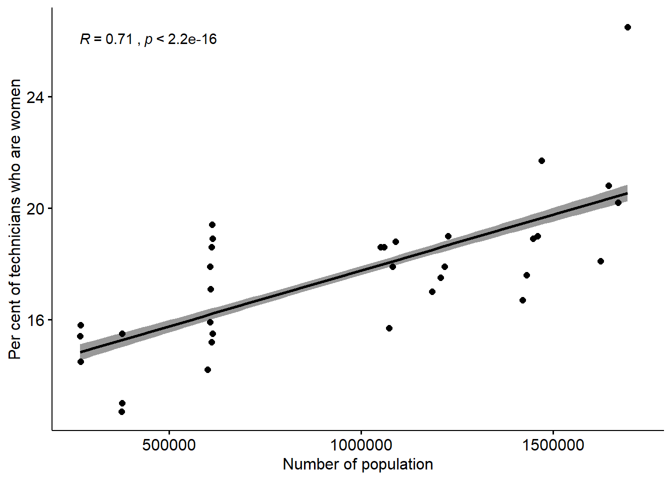
Figure 13.2: The correlation between the proportion of Physical and engineering science technicians who are women and the number of the population in the regions (NUTS2), Year 2014 - 2018.
tb <- readfile("000000CG_12.csv")
tb <- readfile("000000CD_12.csv") %>%
  left_join(tb, by = c("region", "year", "sex")) %>%
  drop_na %>%
  group_by (`region`, year) %>%
  mutate (perc_women = as.numeric (sub ("%", "", perc_women (salary.x)))) %>%
  mutate (perc_salary = as.numeric (sub ("%", "", perc_sal (salary.y)))) %>%
  mutate (sum_ing = sum(salary.x))
tb <- readfile("UF0506A1_1.csv") %>%
  group_by(`level of education`, region, year, sex) %>%
  mutate(utbregno = sum(salary)) %>%
  group_by(region, year, sex) %>% mutate(perc_edu = utbregno / sum(utbregno)) %>%
  group_by(region, year) %>% mutate(sum_pop = sum(utbregno)) %>%
  group_by(`level of education`, region, year) %>%
  mutate (sum_edu = sum(utbregno)) %>%
  right_join(tb, by = c("region", "year", "sex")) %>%
  mutate (perc_eng = sum_ing / sum_edu) %>%
  filter (`level of education` == "post-secondary education 3 years or more (ISCED97 5A)")

model <- lm(perc_women ~ sum_edu + year2 + log(salary.y), data = tb)

summary(model) %>%
  tidy() %>%
  knitr::kable(
  booktabs = TRUE,
caption = 'Women technicians and population with 3 years or more post-secondary education')| term | estimate | std.error | statistic | p.value |
|---|---|---|---|---|
| (Intercept) | -1136.8824353 | 340.1672269 | -3.3421281 | 0.0014129 |
| sum_edu | 0.0000157 | 0.0000021 | 7.5005782 | 0.0000000 |
| year2 | 0.5838037 | 0.1799318 | 3.2445835 | 0.0018973 |
| log(salary.y) | -2.4324403 | 4.4377432 | -0.5481255 | 0.5855739 |
Anova(model, type=2) %>%
  tidy() %>%
  knitr::kable(
  booktabs = TRUE,
caption = 'Anova report from linear model fit') | term | sumsq | df | statistic | p.value |
|---|---|---|---|---|
| sum_edu | 160.7856380 | 1 | 56.2586731 | 0.0000000 |
| year2 | 30.0867780 | 1 | 10.5273222 | 0.0018973 |
| log(salary.y) | 0.8586533 | 1 | 0.3004416 | 0.5855739 |
| Residuals | 177.1941819 | 62 | NA | NA |
13.1 The correlation between the number of Physical and engineering science technicians and the number of the population in the regions, Year 2014 - 2018.
tb <- readfile("000000CG_12.csv")
tb <- readfile("000000CD_12.csv") %>%
 left_join(tb, by = c("region", "year", "sex")) %>%
  drop_na %>%
  group_by (`region`, year) %>%
  mutate (perc_women = as.numeric (sub ("%", "", perc_women (salary.x)))) %>%
  mutate (perc_salary = as.numeric (sub ("%", "", perc_sal (salary.y)))) %>%
  mutate (sum_ing = sum(salary.x))
readfile("UF0506A1_1.csv") %>%
  group_by(`level of education`, region, year, sex) %>%
  mutate(utbregno = sum(salary)) %>%
  group_by(region, year, sex) %>% mutate(perc_edu = utbregno / sum(utbregno)) %>%
  group_by(region, year) %>% mutate(sum_pop = sum(utbregno)) %>%
  group_by(`level of education`, region, year) %>%
  mutate (sum_edu = sum(utbregno)) %>%
  right_join(tb, by = c("region", "year", "sex")) %>%
  mutate (perc_eng = sum_ing / sum_edu) %>%
  ggplot(aes(x = sum_pop, y = sum_ing, colour = region, size = year2)) +
  geom_point() +
  theme(legend.position="bottom") +
  labs(
    x = "Number of population",
    y = "Number of the population who are technicians"
  )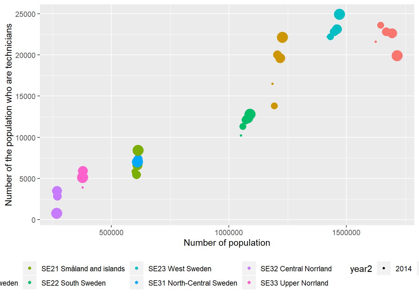
Figure 13.3: The correlation between the number of Physical and engineering science technicians and the number of the population who have 3 years or more post-secondary education, but not postgraduate education in the regions (NUTS2), Year 2014 - 2018.
tb <- readfile("000000CG_12.csv")
tb <- readfile("000000CD_12.csv") %>%
 left_join(tb, by = c("region", "year", "sex")) %>%
  drop_na %>%
  group_by (`region`, year) %>%
  mutate (perc_women = as.numeric (sub ("%", "", perc_women (salary.x)))) %>%
  mutate (perc_salary = as.numeric (sub ("%", "", perc_sal (salary.y)))) %>%
  mutate (sum_ing = sum(salary.x))
readfile("UF0506A1_1.csv") %>%
  group_by(`level of education`, region, year, sex) %>%
  mutate(utbregno = sum(salary)) %>%
  group_by(region, year, sex) %>% mutate(perc_edu = utbregno / sum(utbregno)) %>%
  group_by(region, year) %>% mutate(sum_pop = sum(utbregno)) %>%
  group_by(`level of education`, region, year) %>%
  mutate (sum_edu = sum(utbregno)) %>%
  right_join(tb, by = c("region", "year", "sex")) %>%
  mutate (perc_eng = sum_ing / sum_edu) %>%
  ggscatter(x = "sum_pop", y = "sum_ing",
  add = "reg.line", conf.int = TRUE,
  cor.coef = TRUE, cor.method = "pearson") +
  labs(
    x = "Number of population",
    y = "Number of the population who are technicians"
  )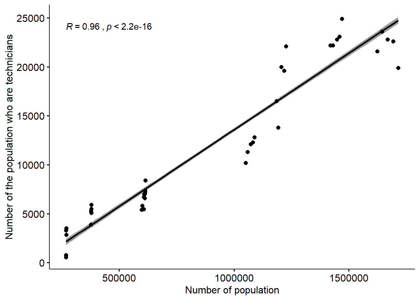
Figure 13.4: The correlation between the number of Physical and engineering science technicians and the number of the population in the regions (NUTS2), Year 2014 - 2018.
13.2 The correlation between the number of Physical and engineering science technicians and the proportion of Physical and engineering science technicians who are women in the regions, Year 2014 - 2018
tb <- readfile("000000CG_12.csv")
tb <- readfile("000000CD_12.csv") %>%
  left_join(tb, by = c("region", "year", "sex")) %>%
  drop_na %>%
  group_by (`region`, year) %>%
  mutate (perc_women = as.numeric (sub ("%", "", perc_women (salary.x)))) %>%
  mutate (perc_salary = as.numeric (sub ("%", "", perc_sal (salary.y)))) %>%
  mutate (sum_ing = sum(salary.x))
readfile("UF0506A1_1.csv") %>%
  group_by(`level of education`, region, year, sex) %>%
  mutate(utbregno = sum(salary)) %>%
  group_by(region, year, sex) %>% mutate(perc_edu = utbregno / sum(utbregno)) %>%
  group_by(`level of education`, region, year) %>%
  mutate (sum_edu = sum(utbregno)) %>%
  right_join(tb, by = c("region", "year", "sex")) %>%
  ggplot(aes(x = perc_women, y = sum_ing, colour = region, size = year2)) +
  geom_point() +
  theme(legend.position="bottom") +
  labs(
    x = "Per cent of technicians who are women",
    y = "Number of the population who are technicians"
  )
## Warning: Removed 56 rows containing missing values (geom_point).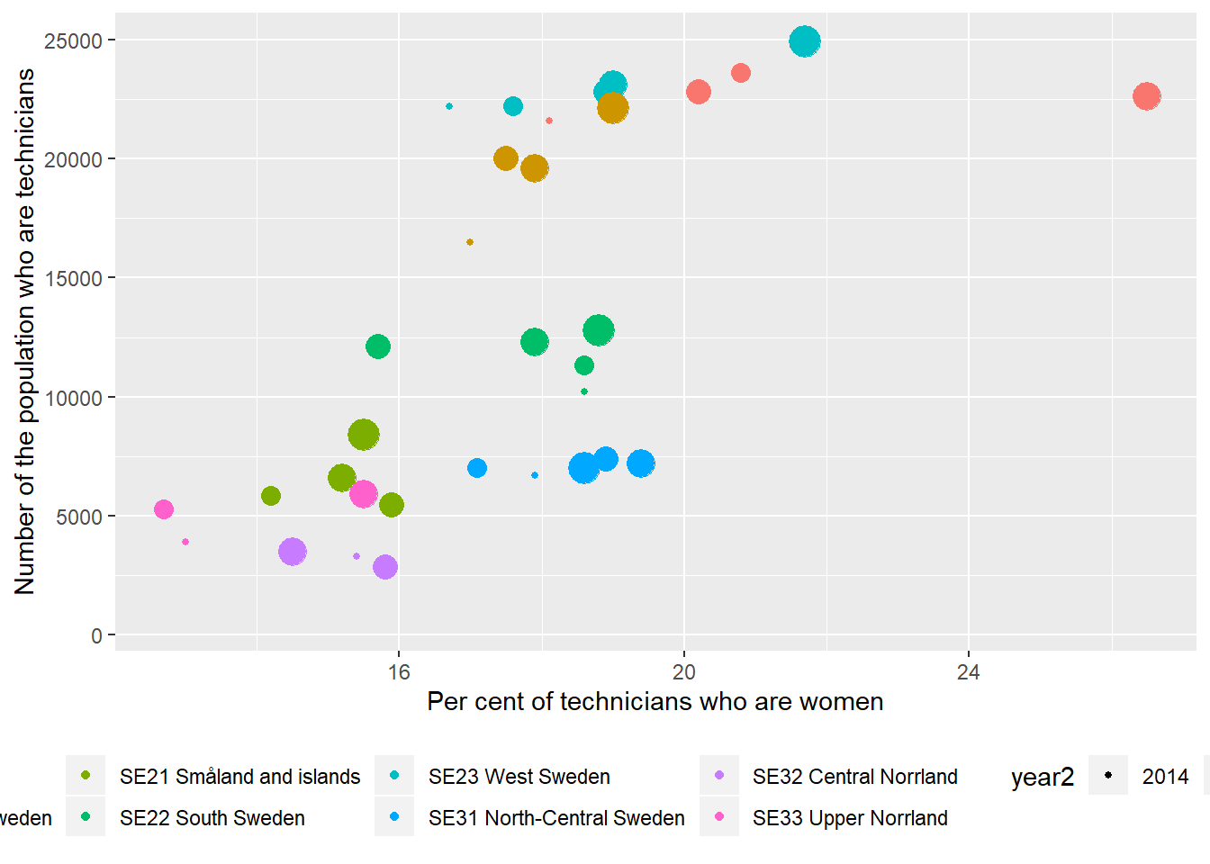
Figure 13.5: The correlation between the number of Physical and engineering science technicians and the proportion of Physical and engineering science technicians who are women in the regions (NUTS2), Year 2014 - 2018.
tb <- readfile("000000CG_12.csv")
tb <- readfile("000000CD_12.csv") %>%
  left_join(tb, by = c("region", "year", "sex")) %>%
  drop_na %>%
  group_by (`region`, year) %>%
  mutate (perc_women = as.numeric (sub ("%", "", perc_women (salary.x)))) %>%
  mutate (perc_salary = as.numeric (sub ("%", "", perc_sal (salary.y)))) %>%
  mutate (sum_ing = sum(salary.x))
readfile("UF0506A1_1.csv") %>%
  group_by(`level of education`, region, year, sex) %>%
  mutate(utbregno = sum(salary)) %>%
  group_by(region, year, sex) %>% mutate(perc_edu = utbregno / sum(utbregno)) %>%
  group_by(region, year) %>%
  mutate (sum_edu = sum(utbregno)) %>%
  right_join(tb, by = c("region", "year", "sex")) %>%
  mutate (perc_eng = sum_ing / sum_edu) %>%
  ggscatter(x = "perc_women", y = "sum_ing",
  add = "reg.line", conf.int = TRUE,
  cor.coef = TRUE, cor.method = "pearson") +
  labs(
    x = "Per cent of technicians who are women",
    y = "Number of the population who are technicians"
  )
## Warning: Removed 56 rows containing non-finite values (stat_smooth).## Warning: Removed 56 rows containing non-finite values (stat_cor).## Warning: Removed 56 rows containing missing values (geom_point).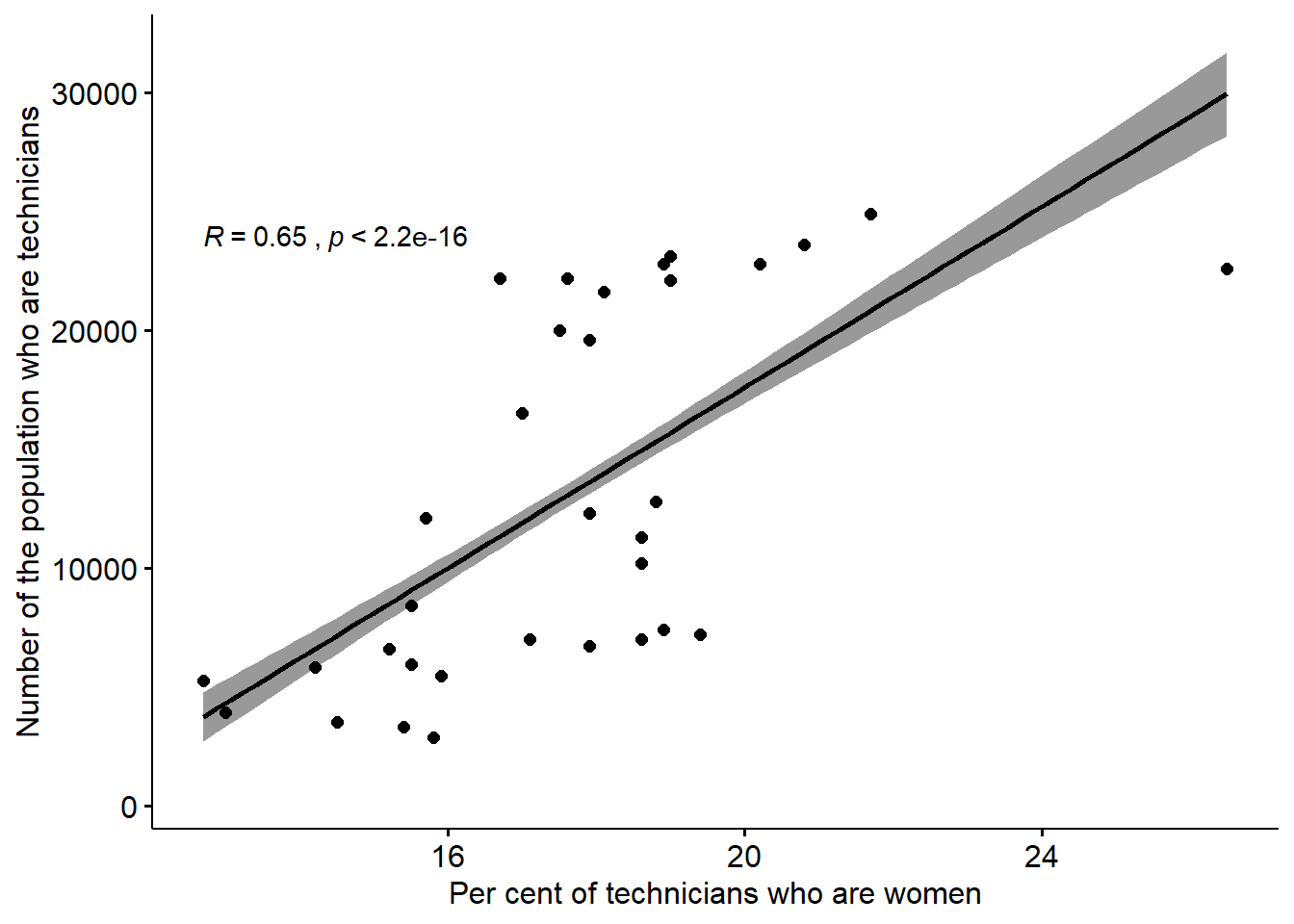
Figure 13.6: The correlation between the number of Physical and engineering science technicians and the proportion of Physical and engineering science technicians who are women in the regions (NUTS2), Year 2014 - 2018.
tb <- readfile("000000CG_12.csv")
tb <- readfile("000000CD_12.csv") %>%
  left_join(tb, by = c("region", "year", "sex")) %>%
  drop_na %>%
  group_by (`region`, year) %>%
  mutate (perc_women = as.numeric (sub ("%", "", perc_women (salary.x)))) %>%
  mutate (perc_salary = as.numeric (sub ("%", "", perc_sal (salary.y)))) %>%
  mutate (sum_ing = sum(salary.x))
tb <- readfile("UF0506A1_1.csv") %>%
  group_by(`level of education`, region, year, sex) %>%
  mutate(utbregno = sum(salary)) %>%
  group_by(region, year, sex) %>% mutate(perc_edu = utbregno / sum(utbregno)) %>%
  group_by(region, year) %>% mutate(sum_pop = sum(utbregno)) %>%
  group_by(`level of education`, region, year) %>%
  mutate (sum_edu = sum(utbregno)) %>%
  right_join(tb, by = c("region", "year", "sex")) %>%
  mutate (perc_eng = sum_ing / sum_edu) %>%
  filter (`level of education` == "post-secondary education 3 years or more (ISCED97 5A)")

model <- lm(sum_ing ~ sum_pop + perc_women + year2 + log(salary.y), data = tb)

summary(model) %>%
  tidy() %>%
  knitr::kable(
  booktabs = TRUE,
caption = 'Engineers and per cent of engineers who are women')| term | estimate | std.error | statistic | p.value |
|---|---|---|---|---|
| (Intercept) | -1.351634e+06 | 4.282187e+05 | -3.156411 | 0.0024818 |
| sum_pop | 1.749690e-02 | 8.714000e-04 | 20.078217 | 0.0000000 |
| perc_women | -3.112504e+02 | 1.453875e+02 | -2.140833 | 0.0362926 |
| year2 | 7.012531e+02 | 2.242318e+02 | 3.127358 | 0.0027027 |
| log(salary.y) | -5.736663e+03 | 5.098312e+03 | -1.125208 | 0.2649087 |
Anova(model, type=2) %>%
  tidy() %>%
  knitr::kable(
  booktabs = TRUE,
caption = 'Anova report from linear model fit') | term | sumsq | df | statistic | p.value |
|---|---|---|---|---|
| sum_pop | 1642189667 | 1 | 403.134815 | 0.0000000 |
| perc_women | 18669754 | 1 | 4.583166 | 0.0362926 |
| year2 | 39840804 | 1 | 9.780366 | 0.0027027 |
| log(salary.y) | 5157495 | 1 | 1.266094 | 0.2649087 |
| Residuals | 248486526 | 61 | NA | NA |
13.3 The correlation between the salary of Physical and engineering science technicians and the number of the population in the regions, Year 2014 - 2018
tb <- readfile("000000CG_12.csv")
tb <- readfile("000000CD_12.csv") %>%
  left_join(tb, by = c("region", "year", "sex")) %>%
  drop_na %>%
  group_by (`region`, year) %>%
  mutate (perc_women = as.numeric (sub ("%", "", perc_women (salary.x)))) %>%
  mutate (perc_salary = as.numeric (sub ("%", "", perc_sal (salary.y)))) %>%
  mutate (sum_ing = sum(salary.x))
readfile("UF0506A1_1.csv") %>%
  group_by(`level of education`, region, year, sex) %>%
  mutate(utbregno = sum(salary)) %>%
  group_by(region, year, sex) %>% mutate(perc_edu = utbregno / sum(utbregno)) %>%
  group_by(region, year) %>% mutate(sum_pop = sum(utbregno)) %>%
  group_by(`level of education`, region, year) %>%
  mutate (sum_edu = sum(utbregno)) %>%
  right_join(tb, by = c("region", "year", "sex")) %>%
  mutate (perc_eng = sum_ing / sum_edu) %>%
  ggplot(aes(x = sum_pop, y = salary.y, colour = region, size = year2)) +
  geom_point() +
  theme(legend.position="bottom") +
  facet_grid(. ~ sex) +
  labs(
    x = "Number of population",
    y = "Salary of engineers"
  )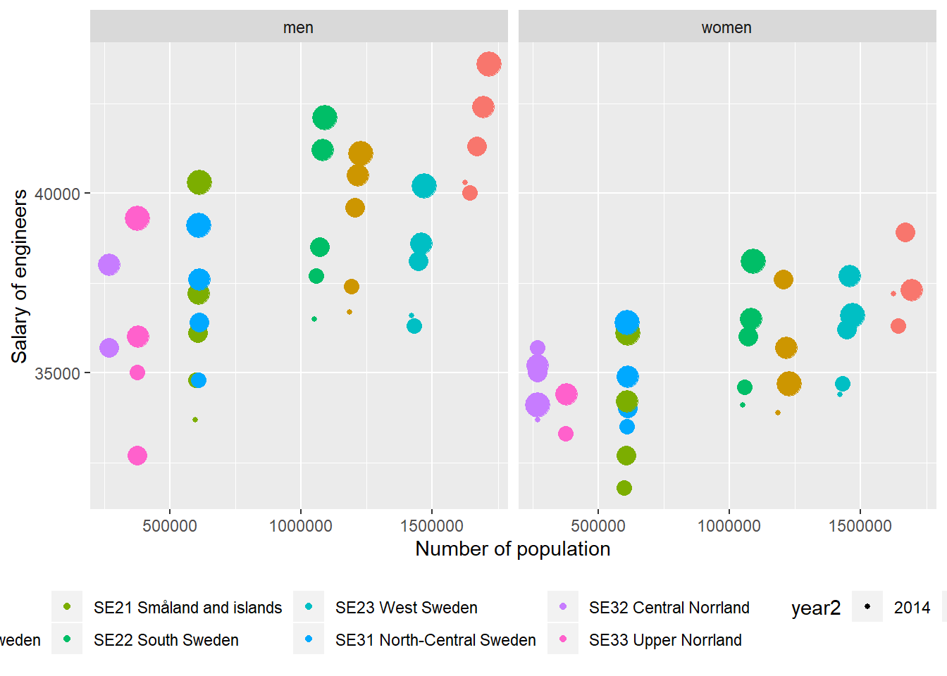
Figure 13.7: The correlation between the salary of Physical and engineering science technicians and the number of the population who have 3 years or more post-secondary education, but not postgraduate education in the regions (NUTS2), Year 2014 - 2018.
tb <- readfile("000000CG_12.csv")
tb <- readfile("000000CD_12.csv") %>%
  left_join(tb, by = c("region", "year", "sex")) %>%
  drop_na %>%
  group_by (`region`, year) %>%
  mutate (perc_women = as.numeric (sub ("%", "", perc_women (salary.x)))) %>%
  mutate (perc_salary = as.numeric (sub ("%", "", perc_sal (salary.y)))) %>%
  mutate (sum_ing = sum(salary.x))
  readfile("UF0506A1_1.csv") %>%
  group_by(`level of education`, region, year, sex) %>%
  mutate(utbregno = sum(salary)) %>%
  group_by(region, year, sex) %>% mutate(perc_edu = utbregno / sum(utbregno)) %>%
  group_by(region, year) %>% mutate(sum_pop = sum(utbregno)) %>%
  group_by(`level of education`, region, year) %>%
  mutate (sum_edu = sum(utbregno)) %>%
  right_join(tb, by = c("region", "year", "sex")) %>%
  mutate (perc_eng = sum_ing / sum_edu) %>%
  ggscatter(x = "sum_pop", y = "salary.y",
  add = "reg.line", conf.int = TRUE,
  cor.coef = TRUE, cor.method = "pearson") +
  facet_grid(. ~ sex) +
  facet_grid(. ~ sex) +
  labs(
    x = "Number of population",
    y = "Salary of technicians"
  )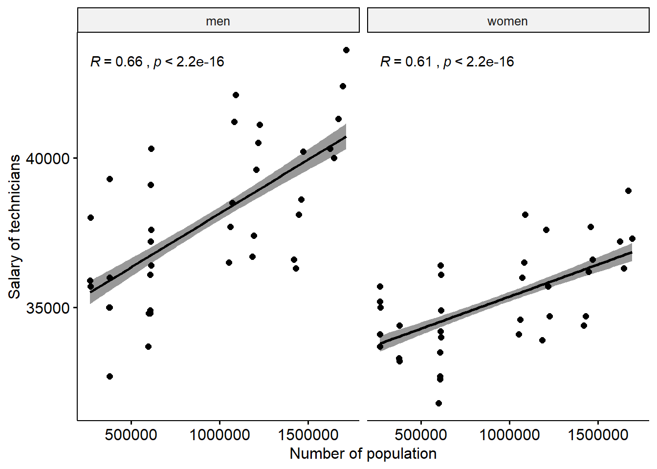
Figure 13.8: The correlation between the salary of Physical and engineering science technicians and the number of the population in the regions (NUTS2), Year 2014 - 2018.
13.4 The correlation between the salary of Physical and engineering science technicians and the number of Physical and engineering science technicians in the regions, Year 2014 - 2018
tb <- readfile("000000CG_12.csv")
tb <- readfile("000000CD_12.csv") %>%
  left_join(tb, by = c("region", "year", "sex")) %>%
  drop_na %>%
  group_by (`region`, year) %>%
  mutate (perc_women = as.numeric (sub ("%", "", perc_women (salary.x)))) %>%
  mutate (perc_salary = as.numeric (sub ("%", "", perc_sal (salary.y)))) %>%
  mutate (sum_ing = sum(salary.x))
readfile("UF0506A1_1.csv") %>%
  group_by(`level of education`, region, year, sex) %>%
  mutate(utbregno = sum(salary)) %>%
  group_by(region, year, sex) %>% mutate(perc_edu = utbregno / sum(utbregno)) %>%
  group_by(region, year) %>% mutate(sum_pop = sum(utbregno)) %>%
  group_by(`level of education`, region, year) %>%
  mutate (sum_edu = sum(utbregno)) %>%
  right_join(tb, by = c("region", "year", "sex")) %>%
  mutate (perc_eng = sum_ing / sum_edu) %>%
  ggplot(aes(x = sum_ing, y = salary.y, colour = region, size = year2)) +
  geom_point() +
  theme(legend.position="bottom") +
  facet_grid(. ~ sex) +
  labs(
    x = "Number of the population who are technicians",
    y = "Salary of technicians"
  )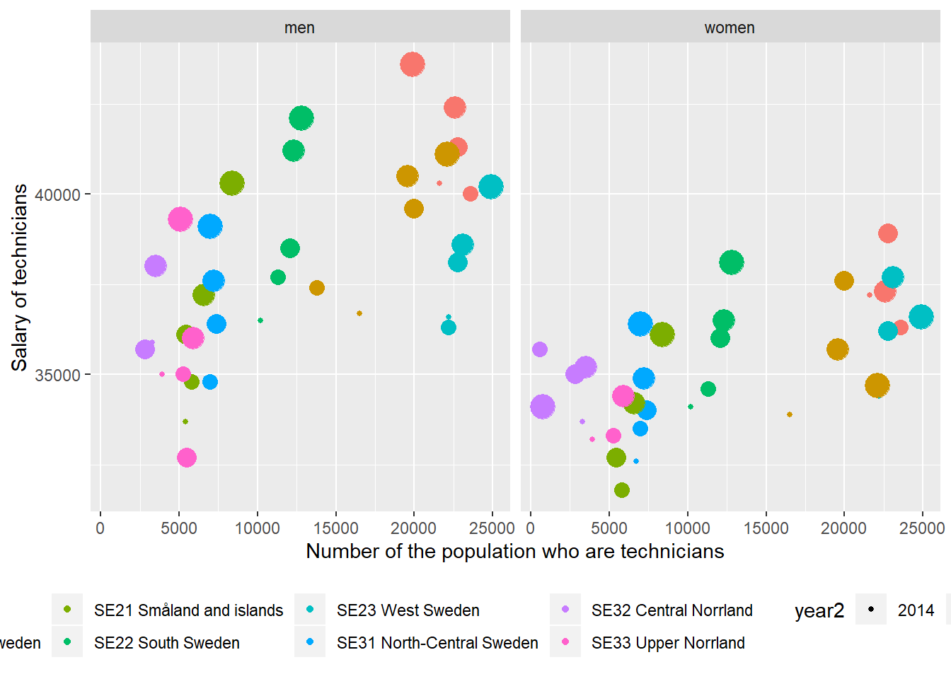
Figure 13.9: The correlation between the number of Physical and engineering science technicians and the number of the population who have 3 years or more post-secondary education, but not postgraduate education in the regions (NUTS2), Year 2014 - 2018.
tb <- readfile("000000CG_12.csv")
tb <- readfile("000000CD_12.csv") %>%
  left_join(tb, by = c("region", "year", "sex")) %>%
  drop_na %>%
  group_by (`region`, year) %>%
  mutate (perc_women = as.numeric (sub ("%", "", perc_women (salary.x)))) %>%
  mutate (perc_salary = as.numeric (sub ("%", "", perc_sal (salary.y)))) %>%
  mutate (sum_ing = sum(salary.x))
  readfile("UF0506A1_1.csv") %>%
  group_by(`level of education`, region, year, sex) %>%
  mutate(utbregno = sum(salary)) %>%
  group_by(region, year, sex) %>% mutate(perc_edu = utbregno / sum(utbregno)) %>%
  group_by(region, year) %>% mutate(sum_pop = sum(utbregno)) %>%
  group_by(`level of education`, region, year) %>%
  mutate (sum_edu = sum(utbregno)) %>%
  right_join(tb, by = c("region", "year", "sex")) %>%
  mutate (perc_eng = sum_ing / sum_edu) %>%
  ggscatter(x = "sum_ing", y = "salary.y",
  add = "reg.line", conf.int = TRUE,
  cor.coef = TRUE, cor.method = "pearson") +
  facet_grid(. ~ sex) +
  labs(
    x = "Number of the population who are technicians",
    y = "Salary of technicians"
  )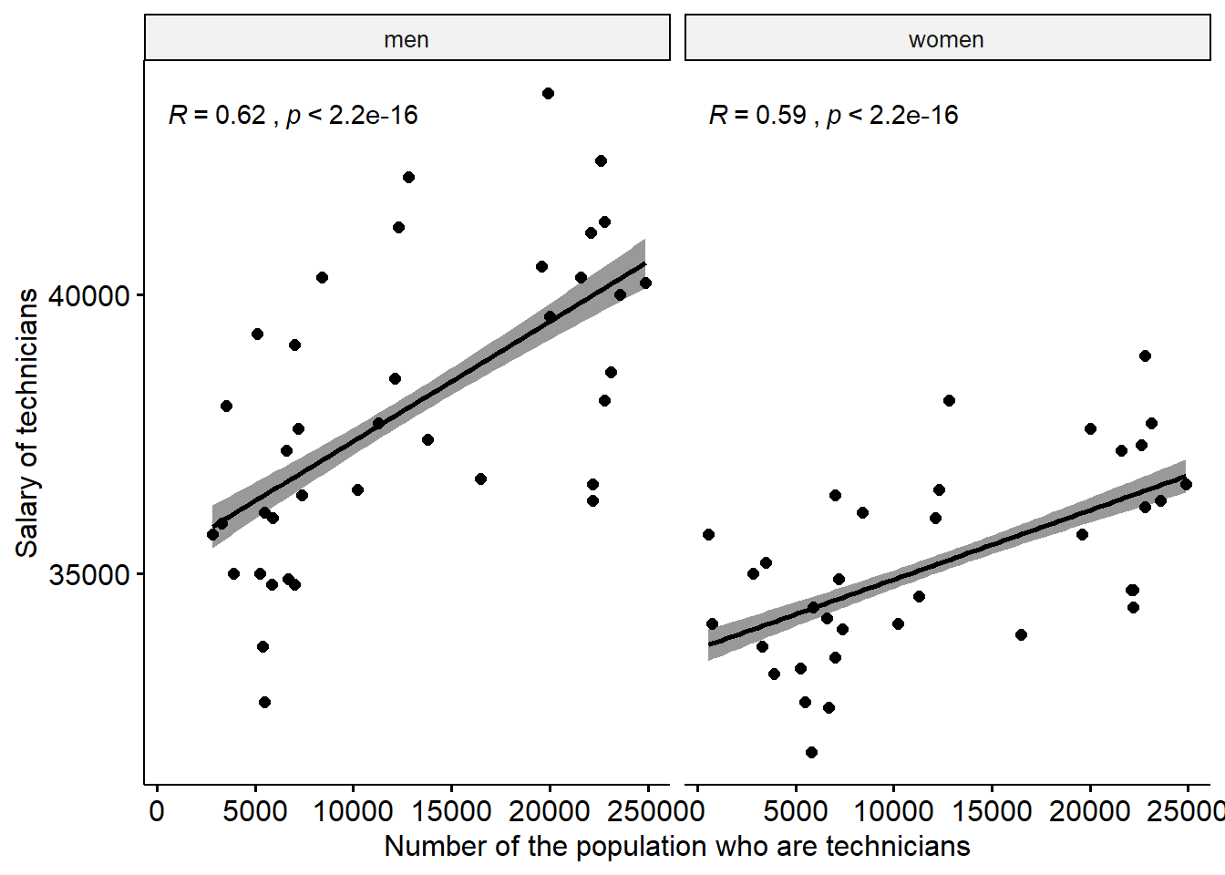
Figure 13.10: The correlation between the salary of Physical and engineering science technicians and the number of Physical and engineering science technicians in the regions (NUTS2), Year 2014 - 2018.
tb <- readfile("000000CG_12.csv")
tb <- readfile("000000CD_12.csv") %>%
  left_join(tb, by = c("region", "year", "sex")) %>%
  drop_na %>%
  group_by (`region`, year) %>%
  mutate (perc_women = as.numeric (sub ("%", "", perc_women (salary.x)))) %>%
  mutate (perc_salary = as.numeric (sub ("%", "", perc_sal (salary.y)))) %>%
  mutate (sum_ing = sum(salary.x))
tb <- readfile("UF0506A1_1.csv") %>%
  group_by(`level of education`, region, year, sex) %>%
  mutate(utbregno = sum(salary)) %>%
  group_by(region, year, sex) %>% mutate(perc_edu = utbregno / sum(utbregno)) %>%
  group_by(region, year) %>% mutate(sum_pop = sum(utbregno)) %>%
  group_by(`level of education`, region, year) %>%
  mutate (sum_edu = sum(utbregno)) %>%
  right_join(tb, by = c("region", "year", "sex")) %>%
  mutate (perc_eng = sum_ing / sum_edu) %>%
  filter (`level of education` == "post-secondary education 3 years or more (ISCED97 5A)")

model <- lm(log(salary.y) ~ sum_edu + year2 + perc_women, data = tb)

summary(model) %>%
  tidy() %>%
  knitr::kable(
  booktabs = TRUE,
caption = 'Salary of engineers and population with 3 years or more post-secondary education')| term | estimate | std.error | statistic | p.value |
|---|---|---|---|---|
| (Intercept) | -35.4037013 | 9.5439646 | -3.7095382 | 0.0004459 |
| sum_edu | 0.0000003 | 0.0000001 | 4.4492512 | 0.0000365 |
| year2 | 0.0227592 | 0.0047449 | 4.7966022 | 0.0000105 |
| perc_women | -0.0019826 | 0.0036170 | -0.5481255 | 0.5855739 |
Anova(model, type=2) %>%
  tidy() %>%
  knitr::kable(
  booktabs = TRUE,
caption = 'Anova report from linear model fit') | term | sumsq | df | statistic | p.value |
|---|---|---|---|---|
| sum_edu | 0.0461122 | 1 | 19.7958366 | 0.0000365 |
| year2 | 0.0535932 | 1 | 23.0073925 | 0.0000105 |
| perc_women | 0.0006998 | 1 | 0.3004416 | 0.5855739 |
| Residuals | 0.1444222 | 62 | NA | NA |